All the image synthesis techniques we have seen thus far have involved either minimizing a convex function or naïvely iterating over a large search space. Now, we move into the world of deep learning: using back propagation to optimize a highly non-convex cascade of affine transforms and non-linearities. While originally used for finding optimal decision surfaces for discriminative tasks, deep neural networks can also act as generative models. We will explore a few such methods in this post.
Generative Adversarial Networks
Let us say that we want to generate new data that is similar in style to an existing set of data. Let us assume that this real data is modeled by an unknown probability distribution p. Since p is unknown, we can’t simply sample new data points from the real distribution.
Instead, let us consider a second known probability distribution over our synthesized data q. Although we don’t know the real distribution p, we can still minimize the expected f-divergence between the real and synthesized distributions. By doing so, we encourage samples drawn from our “fake” distribution q to appear as if drawn from the real distribution p.
For a convex function f such that f(1)=0, the f-divergence between two distributions p and q is defined as
 = \int f\left(\frac{dp}{dq}\right)dq")
Theoretically, Generative Adversarial Networks operate by minimizing this f-divergence between the real and generated distributions. However, they can intuitively be viewed from a game-theoretic approach as well.
Consider two neural networks: the generator g and the discriminator d. The objective of the discriminator can be thought of determining whether a sample comes from the set of real data or from the generator. The objective of the generator is to then generate images that appear like they are from the real data such that they fool the discriminator.
DC-GAN
The Deep Convolutional GAN (DC-GAN) framework builds on the original GAN proposed by Goodfellow et al. by removing the fully connected layers such that every layer of both the generator and discriminator are convolutional (or de-convolutional).
While the original DC-GAN optimizes the Jensen-Shannon Divergence between the real and fake distributions, we use the Least Squares GAN (LS-GAN) loss function that instead optimizes the Pearson 
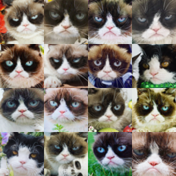
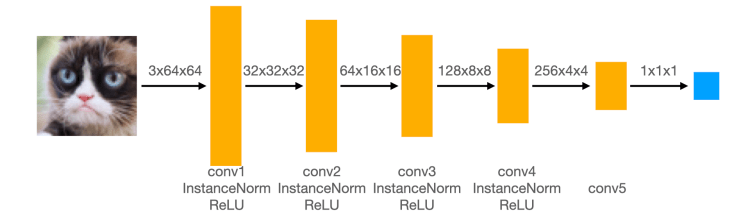
For our experiments, we use a small dataset of 204 grumpy cat images and a relatively shallow architecture for both our generator and discriminator.
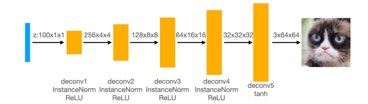
Since our networks are fully convolutional, up/down-sampling is done through strided convolution. Knowing that we want to up/down-sample by a factor of 2, we have the following equation for the size of the output:
/S")
Where K is the size of the filter, W is the size of the input, and S is the stride.
With K=4, S=2, we have that
/2 \implies P=2")
Discriminator
Using the LS-GAN loss, our discriminator loss is defined as
![\displaystyle \mathcal{L}_D = \mathbb{E}_{x\sim data}[(D(x)-1)^2] + \mathbb{E}_{z\sim \mathcal{N}(0,I)}\mathbb{E}[D(G(z))^2]](https://s0.wp.com/latex.php?latex=%5Cdisplaystyle+%5Cmathcal%7BL%7D_D+%3D+%5Cmathbb%7BE%7D_%7Bx%5Csim+data%7D%5B%28D%28x%29-1%29%5E2%5D+%2B+%5Cmathbb%7BE%7D_%7Bz%5Csim+%5Cmathcal%7BN%7D%280%2CI%29%7D%5Cmathbb%7BE%7D%5BD%28G%28z%29%29%5E2%5D+&is-pending-load=1#038;bg=1f2527&fg=ffffff&s=4&c=20201002 "\displaystyle \mathcal{L}_D = \mathbb{E}_{x\sim data}[(D(x)-1)^2] + \mathbb{E}_{z\sim \mathcal{N}(0,I)}\mathbb{E}[D(G(z))^2]")
Generator
Similarly, our generator loss is defined as
![\displaystyle \mathcal{L}_G = \mathbb{E}_{z\sim \mathcal{N}(0,I)}\mathbb{E}[(D(G(z))-1)^2]](https://s0.wp.com/latex.php?latex=%5Cdisplaystyle+%5Cmathcal%7BL%7D_G+%3D+%5Cmathbb%7BE%7D_%7Bz%5Csim+%5Cmathcal%7BN%7D%280%2CI%29%7D%5Cmathbb%7BE%7D%5B%28D%28G%28z%29%29-1%29%5E2%5D+&is-pending-load=1#038;bg=1f2527&fg=ffffff&s=4&c=20201002 "\displaystyle \mathcal{L}_G = \mathbb{E}_{z\sim \mathcal{N}(0,I)}\mathbb{E}[(D(G(z))-1)^2]")
Results
By synchronously training the generator and discriminator during training, we obtain the following loss curves:
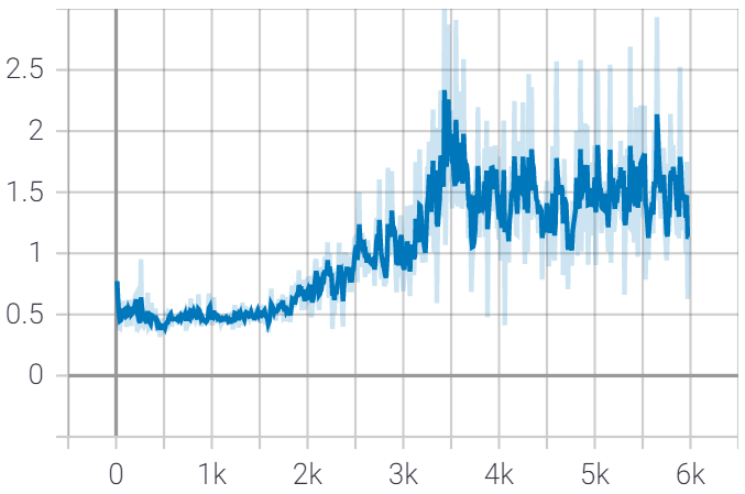
Generator Loss 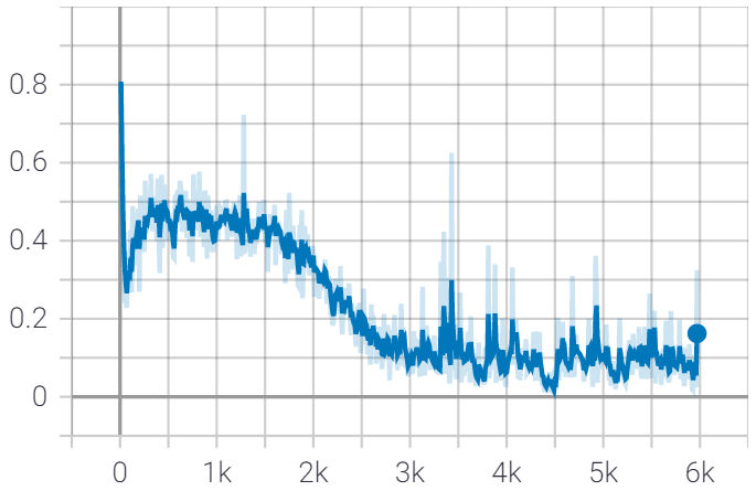
Discriminator Loss
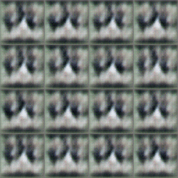
At the end of training, we had the following results sampled from random latent vectors:
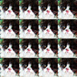
It’s easy to see that these results aren’t great… Not only do the images not look very realistic, but the generator produced the same image for every latent vector.
Observing generated images throughout the training process shows that these issues persist throughout the whole process:
These are both effects of us having a very small training set. To alleviate this, we implement data augmentation to artificially inflate the size of our training set. During training, we now upscale the images before randomly cropping back to the original size and then randomly choose whether or not to perform a horizontal flip.
Applying our data augmentation to the training loop yields the following loss curves (red):
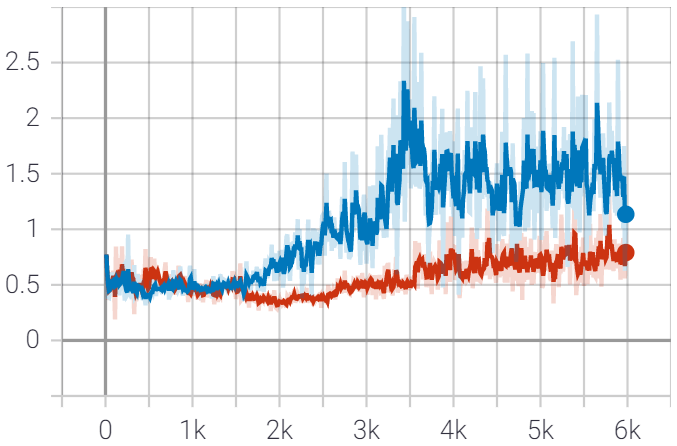
Generator Loss 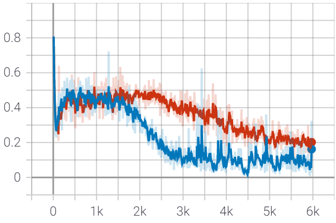
Discriminator Loss
We see that adding data augmentation reduced the generator loss and increases the discriminator loss. This can be interpreted as the generator creating better quality images that better “fool” the discriminator.
In general, the curves for both generator and discriminator loss should oscillate somewhere between 0 and 1 if the GAN manages to train. We don’t want to see curves that are too smooth, as this would indicate either the generator or discriminator is dominating the other.
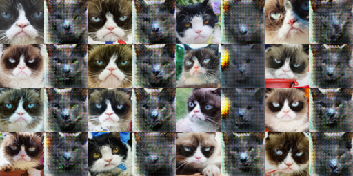
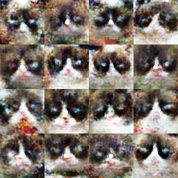
After just 200 iterations using data augmentation, we have the following samples:
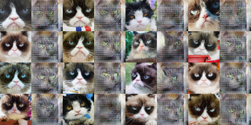
At first glance, it seems like we might be running into the same results as when we did not use data augmentation. However, sampling from random latent vectors after 6000 iterations yields much better results:
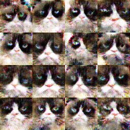
Not only are these images more realistic than those generated without data augmentation (still not perfect), but they are much more diverse as well. Observing the training process also shows that the data augmentation makes the optimization much more stable:
Throughout training, we see the samples transform from noisy blobs to more realistic looking Grumpy Cats.
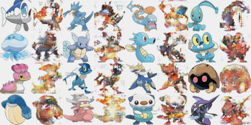
We can also apply our DC-GAN to generate new images of Pokémon from a set of samples.
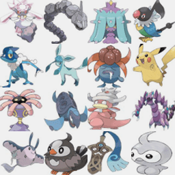
After training for many times more iterations than on the Grumpy Cat dataset, we get the following as our best results:
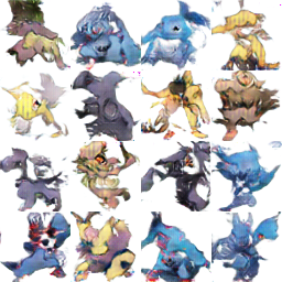
However, after just a few hundred more iterations, we see a large spike in generator loss followed by the GAN collapsing, resulting in the following images:
The entire training process can be viewed below:
CycleGAN
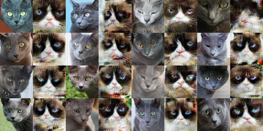
We can also use the GAN paradigm to “translate” between two different styles of images. Here, we will implement CycleGAN to translate Grumpy Cats (N=204) to Russian Blues (N=75) and vice versa. To do this, we create two discriminators (one for each class) and a generator for each direction where rather than a random latent vector, the generator’s input is a sample from the source class:
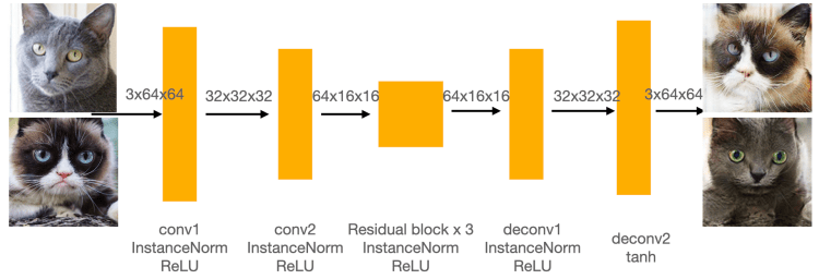
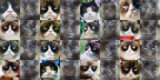
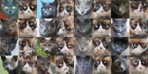
Training our CycleGAN yields the following results. Results are shown in column pairs. The left column shows the CycleGAN input, and the right column is the “translated” fake image.
After just 400 iterations, the CycleGAN’s output is still quite blurry:
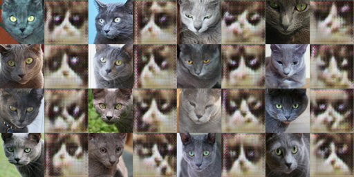
Once we train for 10000 iterations in total, the results become much clearer.
As before, we also include intermediate results to visualize the training process:

Cycle Consistency Loss
On its own, the images generated by CycleGAN may not necessarily look like direct translations of the inputs. We can have preservation of content by encouraging the two generators to be (pseudo)inverses of each other such that they must preserve as much information from the input as possible. We do this by adding a Cycle Consistency Loss to each of the generators:
![\displaystyle \mathcal{L}_{cycle}^{(X\to Y\to X)} = \mathbb{E}_{y\sim Y}[\|y - G_{X\to Y}(G_{Y\to X}(y))\|_p]](https://s0.wp.com/latex.php?latex=%5Cdisplaystyle+%5Cmathcal%7BL%7D_%7Bcycle%7D%5E%7B%28X%5Cto+Y%5Cto+X%29%7D+%3D+%5Cmathbb%7BE%7D_%7By%5Csim+Y%7D%5B%5C%7Cy+-+G_%7BX%5Cto+Y%7D%28G_%7BY%5Cto+X%7D%28y%29%29%5C%7C_p%5D+&is-pending-load=1#038;bg=1f2527&fg=ffffff&s=4&c=20201002 "\displaystyle \mathcal{L}_{cycle}^{(X\to Y\to X)} = \mathbb{E}_{y\sim Y}[\|y - G_{X\to Y}(G_{Y\to X}(y))\|_p]")
By incorporating the Cycle Consistency Loss into our training, we get the following results.
Once again, training for just 400 iterations yields quite blurry results:
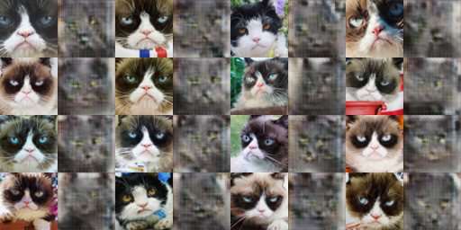
Training for 10000 iterations yields much clearer results for the generated Grumpy Cats although the generated Russian Blues remain very blurry:
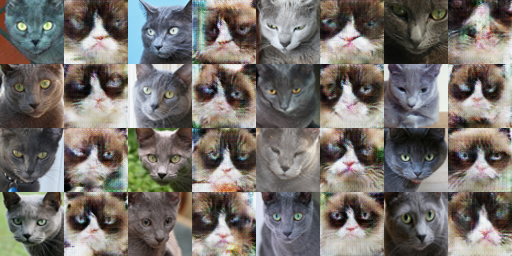
While the quality of the images themselves (especially the generated Blue Russians) is not as good while using the Cyclic Loss, we see that the generated images better capture the pose and orientation of the source. This is because the optimization now also puts weight onto the Cycle Consistency Loss, forcing the generators to become each others’ inverses and preserve information. In doing so, it was not able to put as much “effort” into fooling the generator. However, both of these problems would likely be resolved by using larger datasets; both the Grumpy Cat and Russian Blue dataset are very small.
Again, the training processes are shown below:
We also use our CycleGAN to translate between Fire and Water type Pokémon, although these suffer even more from the small data issue since the set is already so diverse:
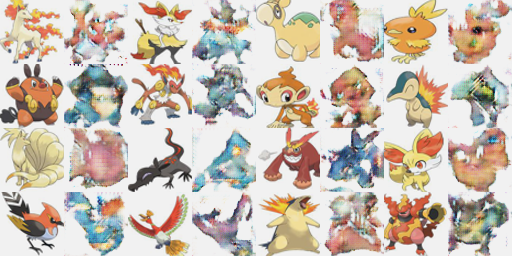
As usual, we also include intermediate results to help visualize the training process:
Wasserstein-GAN
A major problem with the original GAN formulation was that the discriminator would quickly converge to optimality, resulting in vanishing gradients for the generator. While the LS-GAN loss helps to alleviate this, we will explore another such method here: the Wasserstein GAN.
By restricting the Lipschitzness (steepness) of the discriminator, we can then optimize the Wasserstein (or “Earth-Mover”) distance between the real and generated distributions:
![\displaystyle W_1(p\|q) = \max_{f \in F}|\mathbb{E}_p[f(p)] - \mathbb{E}_q[f(q)]|](https://s0.wp.com/latex.php?latex=%5Cdisplaystyle+W_1%28p%5C%7Cq%29+%3D+%5Cmax_%7Bf+%5Cin+F%7D%7C%5Cmathbb%7BE%7D_p%5Bf%28p%29%5D+-+%5Cmathbb%7BE%7D_q%5Bf%28q%29%5D%7C+&is-pending-load=1#038;bg=1f2527&fg=ffffff&s=4&c=20201002 "\displaystyle W_1(p\|q) = \max_{f \in F}|\mathbb{E}_p[f(p)] - \mathbb{E}_q[f(q)]|")
 \leq 1\}")
Here, we use the gradient penalty technique to encourage the gradients of the discriminator to be close to 1 (implying 1-Lipschitzness):
![\displaystyle \mathcal{L}_{GP} = \lambda \mathbb{E}_{\hat{x}}[(\|\nabla_{\hat{x}} D(\hat{x})\|_2-1)^2]](https://s0.wp.com/latex.php?latex=%5Cdisplaystyle+%5Cmathcal%7BL%7D_%7BGP%7D+%3D+%5Clambda+%5Cmathbb%7BE%7D_%7B%5Chat%7Bx%7D%7D%5B%28%5C%7C%5Cnabla_%7B%5Chat%7Bx%7D%7D+D%28%5Chat%7Bx%7D%29%5C%7C_2-1%29%5E2%5D+&is-pending-load=1#038;bg=1f2527&fg=ffffff&s=4&c=20201002 "\displaystyle \mathcal{L}_{GP} = \lambda \mathbb{E}_{\hat{x}}[(\|\nabla_{\hat{x}} D(\hat{x})\|_2-1)^2]")
Because the Wasserstein metric is continuous and differentiable on 1-Lipschitzness functions, we can train our discriminator to convergence without saturating it and losing gradients for our generator. In practice, we train our discriminator for several iterations between each generator update.
The best results on Grumpy Cat and Pokémon are shown below
W-GAN: Grumpy Cat 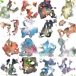
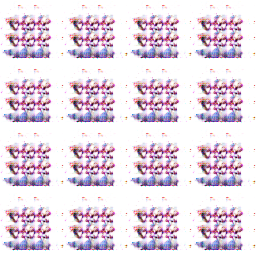
W-GAN: Pokémon
The results here do look noticeably worse than the best results obtained from our JS-GAN. This is likely because our training sets were very small, and the Wasserstein metric requires more data to produce realistic data since the generator no longer has the specific “goal” of “fooling” the discriminator.
However, if we observe the training process, we can see that the W-GAN is much more stable than the JS-GAN. This makes sense due to the required Lipschitzness of the discriminator imposed by the gradient penalty.
W-GAN Training: Grumpy Cat .gif)
W-GAN Training: Pokémon
Variational AutoEncoders
Another deep generative model that does not employ the adversarial approach is the Variational AutoEncoder. This method first assumes that the data are generated by a distribution pθ(x|h) and that the encoder is learning an approximation q𝜙(h|x) to the posterior distribution pθ(h|x). Here, 𝜃 are the parameters of the encoder and 𝜙 are the parameters of the decoder.
We train this model by minimizing the marginal negative log-likelihood of the data by minimizing the negative Evidence Lower Bound (ELBO):
![\displaystyle -ELBO(\theta, \phi; x) = D_{KL}(q_\phi(z|x)\|p_\theta(z)) - \mathbb{E}_{q_\phi(z|x)}[\log p_\theta(x|z)]](https://s0.wp.com/latex.php?latex=%5Cdisplaystyle+-ELBO%28%5Ctheta%2C+%5Cphi%3B+x%29+%3D+D_%7BKL%7D%28q_%5Cphi%28z%7Cx%29%5C%7Cp_%5Ctheta%28z%29%29+-+%5Cmathbb%7BE%7D_%7Bq_%5Cphi%28z%7Cx%29%7D%5B%5Clog+p_%5Ctheta%28x%7Cz%29%5D+&is-pending-load=1#038;bg=1f2527&fg=ffffff&s=3&c=20201002 "\displaystyle -ELBO(\theta, \phi; x) = D_{KL}(q_\phi(z|x)\|p_\theta(z)) - \mathbb{E}_{q_\phi(z|x)}[\log p_\theta(x|z)]")
where DKL is the Kullback–Leibler Divergence, an example of an f-divergence. Here, the KL-divergence measures the distance between the posterior distribution of the latent variable (z) and its prior distribution and is known as the “regularization” loss. Typically, we assume the prior distribution to be a standard multi-variate Gaussian: N(0, I).
The second term of the loss is essentially the cross-entropy between the data and their reconstructions, known as the “reconstruction” loss.
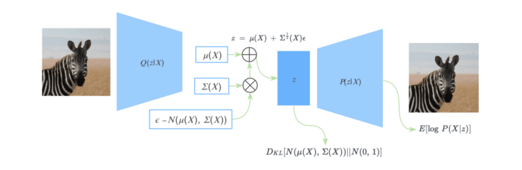
By sampling random vectors from the prior distribution and feeding them through the decoder, we can effectively sample from the approximated data distribution.
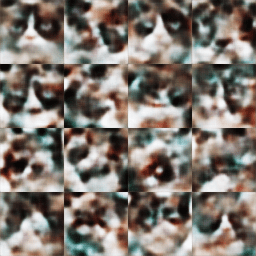
VAE: Grumpy Cat 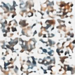
VAE: Pokémon
The results of the Variational AutoEncoder (especially the Pokémon) are mostly just amorphous blobs. However, it still seems feasible that the same distribution that generated these blobs could have generated our very small training sets. With larger training sets, we would have likely seen much clearer results.
Variational AutoEncoders also have an advantage over GANs in that they do not rely on the adversarial paradigm, making them easier to train. They can also be used to disentangle the latent variables used to generate the distribution into the natural independent variables used to generate the real images.
Our final training visualizations can be seen below:
VAE Training: Grumpy Cat 
VAE Training: Pokémon

I’m enjoying these. Do you guys use pytorch? Or tensorflow? Or do you just generate these from the ground up?