If you’re viewing this at cmu.edu, please visit georgecazenavette.com/blog to view in the intended layout 
In this post, we will explore copying a section from a “source” image and blending it into the background of a “target” image. If we naïvely copy and paste the source pixels into the target image, the product will look very unnatural with harsh borders around the copied area. To make the blending seamless, we will utilize a method of gradient domain fusion called Poisson Blending.
Naïve Stitching
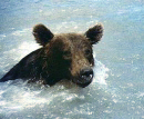
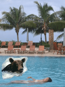
Say we want to take this image of a swimming bear (source image):
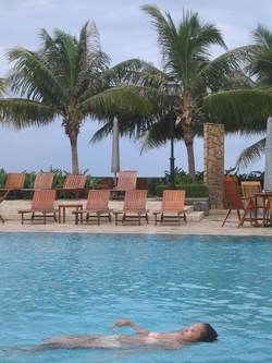
and insert it into this picture of a swimming pool (target image):
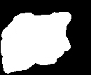
We can create a mask to isolate the subject of interest from the source image
And create a naïve composite image using the following simple formula:
\circ T + M\circ S")
resulting in this poorly blended image:
This composite image looks very unnatural; we can clearly see which pixels were copied over from the source image. What can we do to smooth this boundary between source and target while preserving the content of the copied image?
Poisson Image Editing
Following this paper, we will implement a gradient-based method of image stitching that preserves smoothness over the boundary of the pasted patch. Let Ω be the sub domain of a function f* over which we want to solve for an interpolation function f. We want the interpolation function to equal the original function at the boundary of the patch (denoted ∂Ω), and we also want the gradient of the interpolation function to approximate a guidance vector field, v. This gives us the following optimization problem:

Generalizing to discrete space, the solution to this optimization problem translates to the least-squares solution to the following system of linear equations:

where Np is the set of neighbors of location p. If we set our guidance vector to the gradient of the source patch (v = ∇g), the least squares solution to this system will ensure smoothness at the border also preserving the content of the source.
Toy Problem
Creating and solving this least-squares problem is largest component of Poisson Image Editing. To ensure the correctness of our implementation, we will establish a toy problem where we reconstruct an image using its gradient and one anchor point to solve for the initial condition). I like to think of this problem as using Euler’s Method of solving differential equations.
Using the systems of equations in the previous section, we can set up a sparse least-squares problem of the form

Solving this system gives the following reconstruction:
The fact the the original image and its reconstruction look the same indicates that our implementation functions properly
Poisson Blending
Now that our Discrete Poisson Solver works, we can start experimenting with some seamless cloning. In the first section, we saw that a naïve stitching looks like. Using the same source, mask, and target with our Poisson Solver, we get the following output:
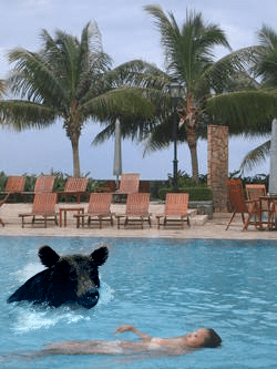
We clearly have a much better composite image than in the naïve setting. The absolute color of the bear may have changed to accommodate a smooth border, but the gradient of the stitched bear matches that of the source image.
We will now show some more examples, of source, target, naïve blend, and Poisson blend:
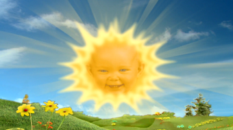
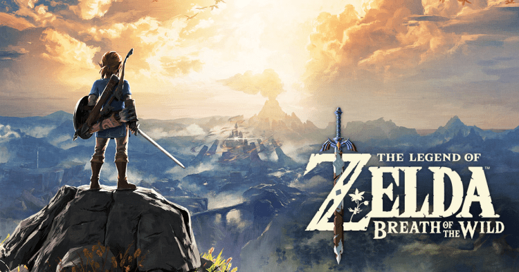
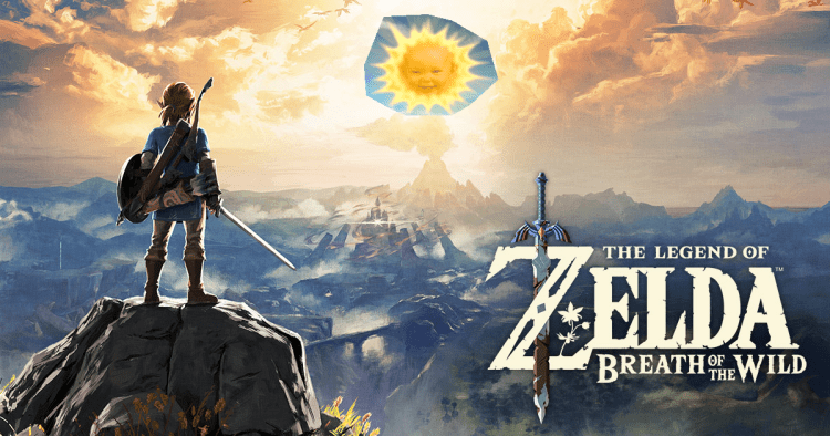
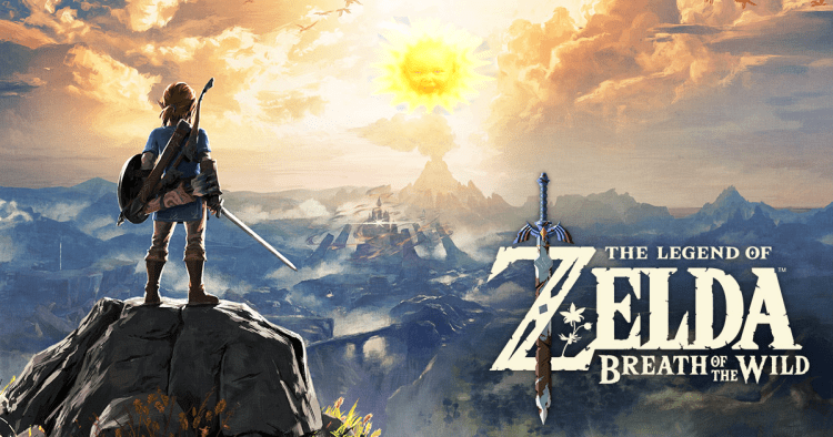
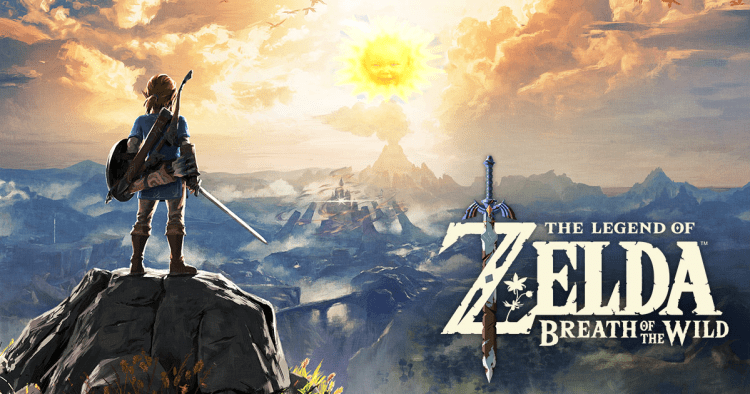
Sunrise over Death Mountain
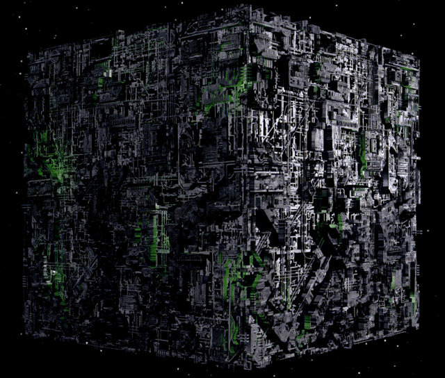
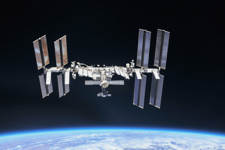
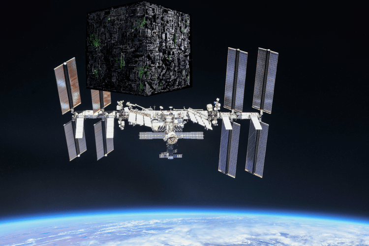
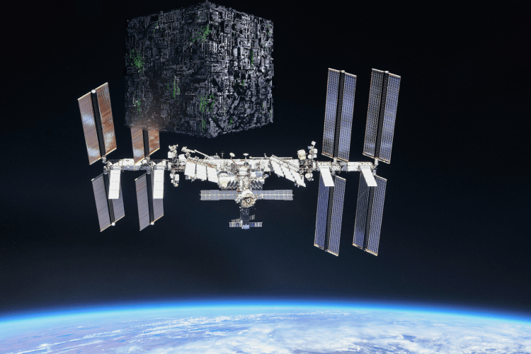
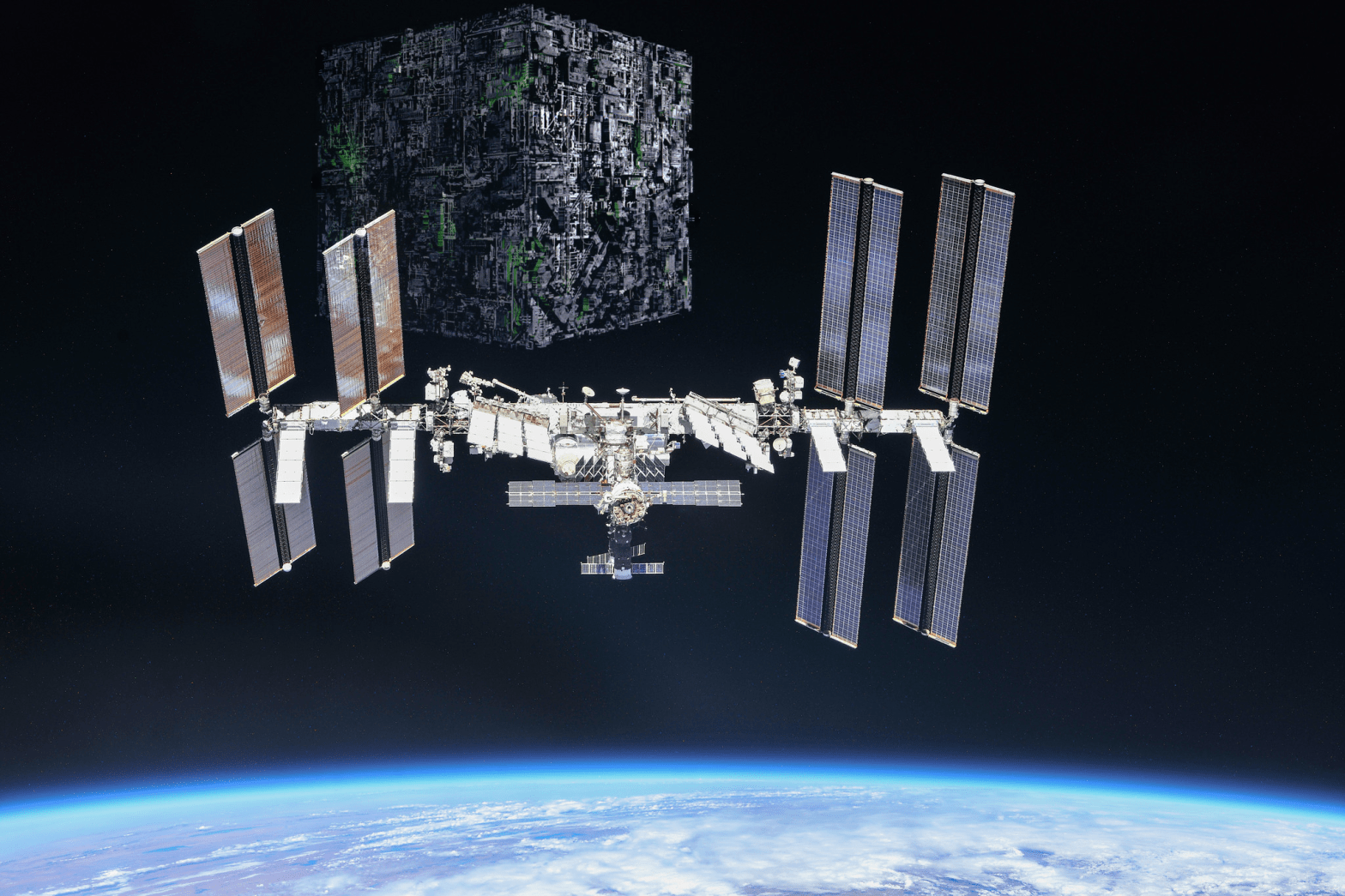
Resistance is Futile
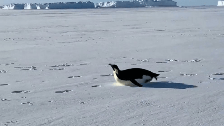
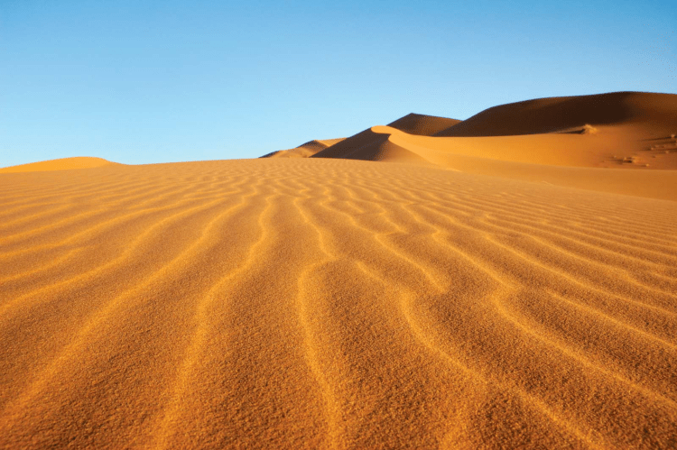
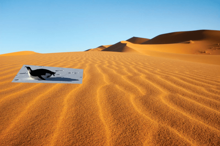
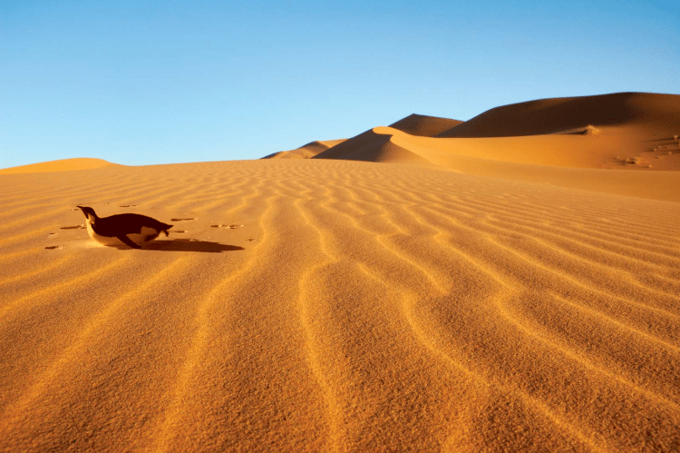
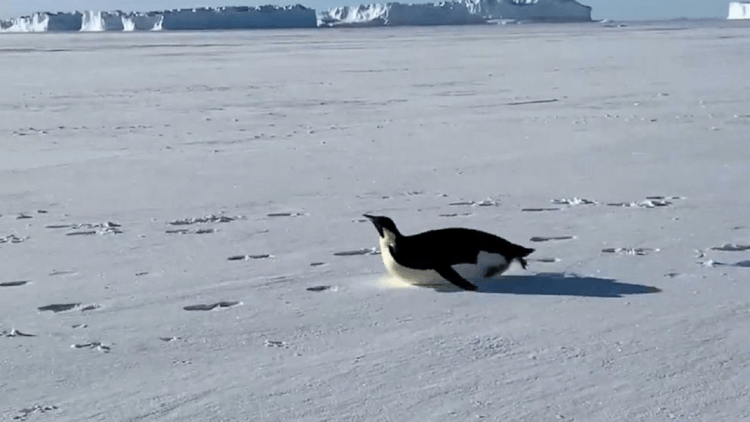
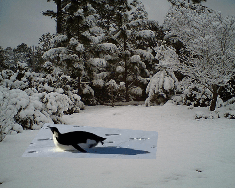
Desert Penguin
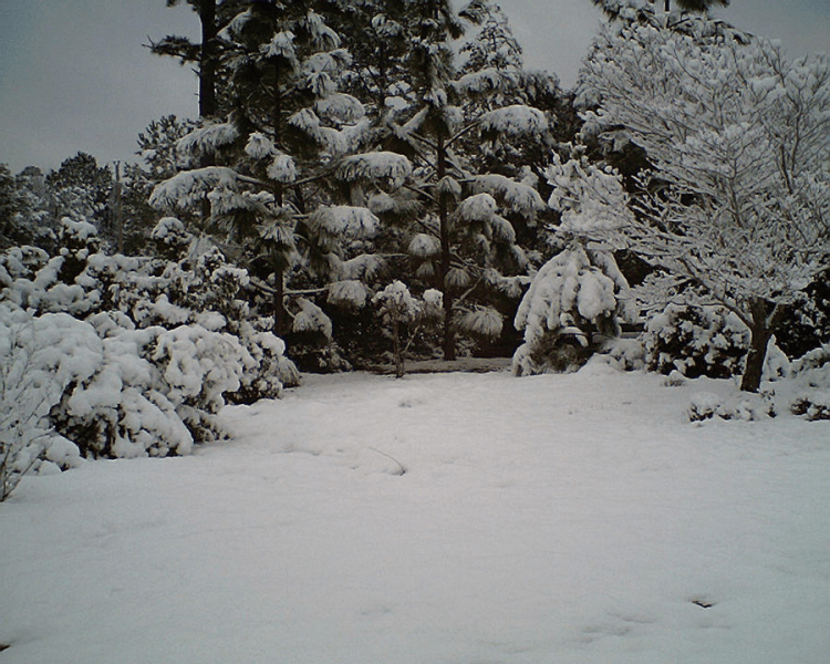
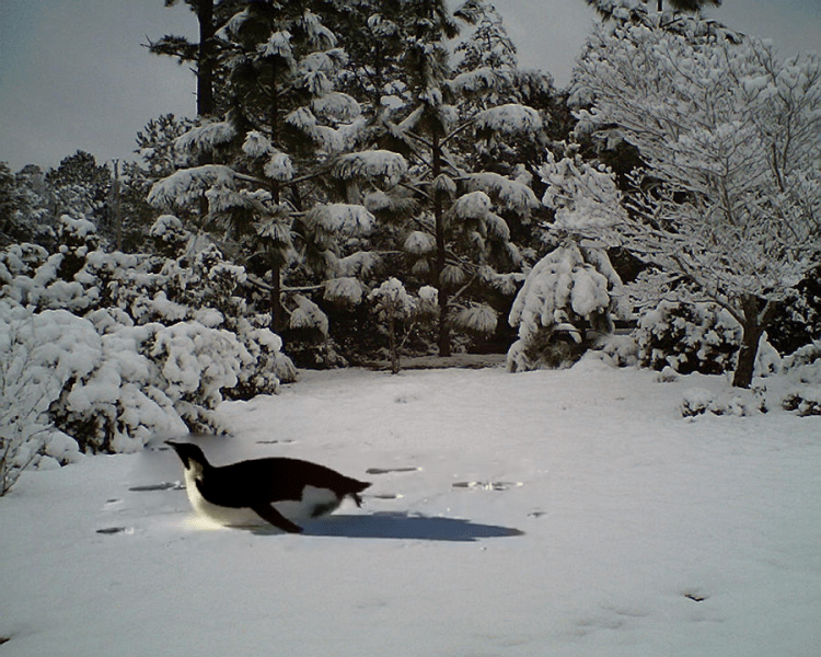
Forest Penguin
In the Star Trek picture, we would ideally want the Borg Cube to be “behind” the ISS along the viewing axis. In the Desert Penguin picture, you can see that the “waves” in the sand have been overwritten in the area surrounding the pasted penguin. In the Forest Penguin picture, we can see a shadowy artifact around the penguin’s head as it blends into the shrub. These are all drawbacks of only using the source gradient as the guidance field.
Mixing Gradients
As we saw in the desert penguin image, interesting information in the target image may sometimes be overwritten by uninteresting gradients from the source image. No handle this, we can make our guidance vector field non-conservative (i.e. not the gradient of some function) and setting it to be whichever either the gradient of the source or target, whichever one has the larger magnitude. This allows us to preserve interesting information from the target as well. We see that this mostly improves the quality of our results:

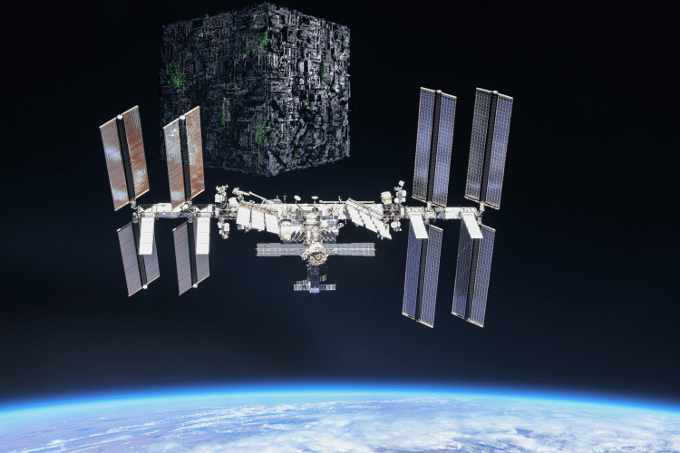

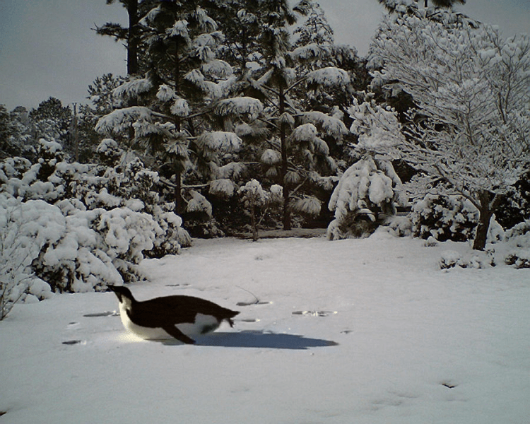
Mixing gradients solved nearly all of the problems with vanilla Poisson Blending. The Borg Cube is now behind the ISS, the waves in the sand behind the Desert Penguin have returned, and the shadowy artifact around the Forest Penguin’s head is gone. However, in some cases, large gradients in the source can overwrite the subject of the patch. For example, you can see sand waves on the Desert Penguin’s body.
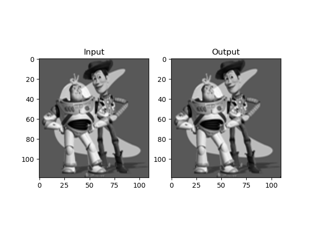
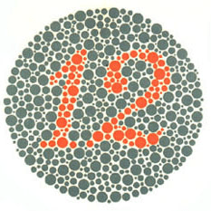
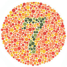
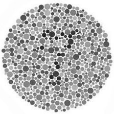
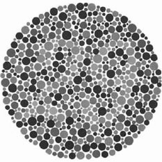
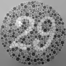
High Contrast Grayscale
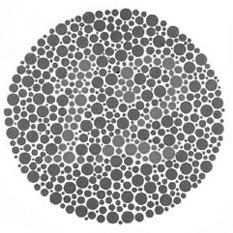
Another usage of gradient domain processing is preserving contrast in grayscale images. Classically, grayscale images are created by simply taking the mean of the red, green, and blue channels. However, this can often result in a loss of contrast:
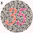
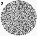
However, we can use our Poisson Solver and creatively choose our guidance vector field to preserve contrast in our resultant image. If we use the method of mixing gradients between the saturation and mean of the RGB channels, we get the following results (right):
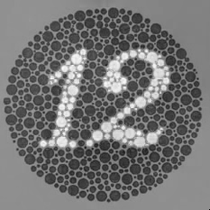
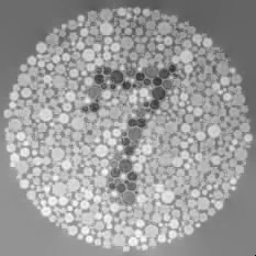
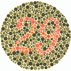
In this way, we can still preserve the content of the original image while only using one channel of information.
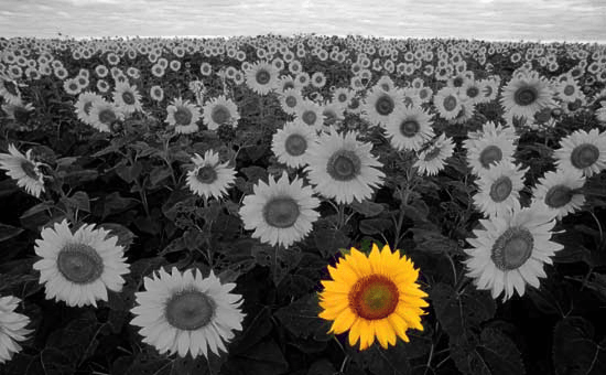
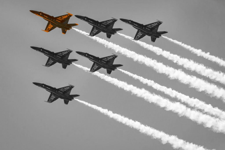
Color Editing
We can also use use Poisson Image Editing to selectively edit the colors of a single image. By setting the target to a grayscale version of the image and using a patch from the color version as our source, we can selectively color only the object selected by the mask.
Left: Naïve Color Selection
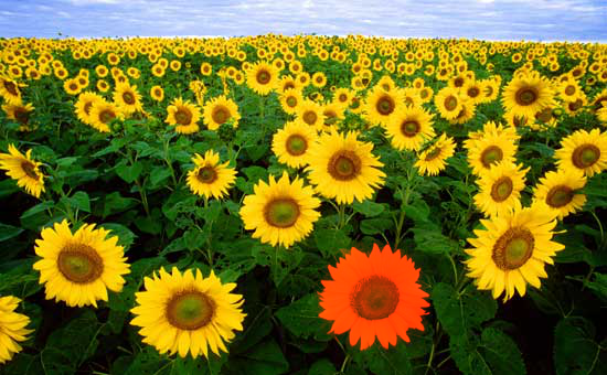
We can also selectively recolor parts of an image by setting the target to the original image and the source as the recolored version:
Thanks for reading!