Physical Clock
In centralized systems, where one or more processors share a common bus, time isn't much of a concern. The entire system shares the same understanding of time: right or wrong, it is consistent.In distributed systems, this is not the case. Unfortunately, each system has its own timer that drives its clock. These timers are based either on the oscillation of a quartz crytal, or equivalent IC. Although they are reasonably precise, stable, and accurate, they are not perfect. This means that the clocks will drift away from the true time. Each timer has different characteristics -- characteristics that might change with time, termperature, &c. This implies that each systems time will drift away from the true time at a different rate -- and perhaps in a different direction (slow or fast).
How Often Do We Need To Resynchronize Clocks?
Coordinating physical clocks among several systems is possible, but it can never be exact. In distributed systems, we must be willing to accept some drift away from the "real" time on each clock.A typical real-time clock within a computer has a relative error of approxmiately 10-5. This means that if the clock is configured for 100 ticks/second, we should expect 360,000 +/- 4 ticks per hour. The maximum drift rate of a clock is the maximum rate at which it can drift.
Since different clocks can drift in different directions, the worst case is that two clocks in a system will drift in opposite directions. In this case the difference between these clocks can be twice the relative error. Use our example relative error of 10-5, this suggests that clocks can drift apart by up to 8 ticks/hour. So, for example, if we want all clocks in this system to be within 4 ticks, we must synchronize them twice per hour.
A general formula expressing these ideas follows:
largest_synchronization_interval = maximum_acceptable_difference/maximum_drift_rate/2
Cristian's Algorithm
Cristian's Algorithm is one approach to synchronizing physical clocks using a time server. The time server is a special host that contains the reference time -- the time that is considered to be (most) correct. Typically time servers are themselves synchronized against another source, such as a UTC time server based on an atomic clock.Cristian's algorithm is a client-pull mechanism. Clients ask the time server for the current time. When the server's response is received, the client tries to adjust it for the transit delay, and then adjusts its own clock.
To understand the reason that the adjustment for the transit time is needed, please remember that the time server is replying with the current time as of the time that it received the request -- not the time that the request was dispatched and not the time that the reply was received by the client.
In order to better estimate the current time, the host needs to estimate how long it has been since the time server replied. Typically this is done by assuming that the client's time is reasonably accurate over short intervals and that the latency of the link is approximately symmetrical (the request takes as long to get to the server as the reply takes to get back). Given these assumtions, the client can measure the round trip time (RTT) of the request using its local clock, divide this time in half, and subtract the local time from the result. The result is a good estimate of the error in the local time. In other words:
local_clock_error = server_timestamp + (response_received_timestamp - request_dispatched_timestamp)/2local_clock_error = server_timestamp + (RTT/2)
If the server is known to have an approximatable latency in answering the requests once it receives them, an adjustment can also be made for this.
local_clock_error = server_timestamp + (RTT - server_latency)/2These estimates can be further improved by adjusting for unusually large RTTs. Long RTTs are likely to be less symmetric, making the estimated error less accurate. One approach might be to keep track of recent RTTs and repeat requests if the RTT appears to be an outlier. Another approach is to use an adaptive average to weight the new estimate of the error against aggregate of prior weighted averages:
avg_clock_error0 = local_clock_error
avg_clock_errorn = (weight * local_clock_error) + (1 - weight) * local_clock_errorn-1If the local clock is slower than the reference clock, the new time value can simply be adopted -- in general, clocks can be advanced without causing many problems. But if the local clock is fast, adopting a prior time is probably not a good idea. Doing so could reverse the apparent order of some events by giving a lower timestamp to an event than a predecessor. In the case of a fast local clock, the clock should be slowed down -- the time should not be adjusted.
Berkeley Algorithm
The Berkeley Algorithm is an approach that is applicable if not time server is available. This approach is somewhat centralized. One active server polls all machines, adjusts them based on the RTT and service time (if known), computes an average, and then tells each server to speed up or to slow down. The average time may be a better estimate of real time than the clock of any one host, but it will still drift. The period of the polling needs to be set as it was before to ensure that the maximum drift in between adjustments is acceptable.
Berkeley Algorithm w/Broadcast
Instead of polling the active server could broadcast to all servers periodically. At the end of the same period, it could collect those times that it received, discard outliers, make the same adjustments for RTT and I as before, and then tell the hosts to adjust their clocks as with Berkeley or Cristian's. At the end of the period, the whole thing is repeated. As with the Berkeley approach, the average time can drift away from the "real time," and the period needs to be sufficiently small to ensure an acceptable level of relative drift.
Multiple Time Servers
If multiple time servers are available, a scheme similar to the Berkeley approach or the variation above can be used to better adjust for the inaccuracy instituted by the RTT-based estimation and to remain more resiliant in the event of failure.
Real-world Synchronization: NTP
Clock synchronization in the real world is based on techniques like the two we just described, but often includes additional statistical filtering and a more complex model for finding a time server. In addition, security becomes a concern -- it is necessary to prevent a malicious user from polluting the reference time.
Logical Clocks
In distributed systems, it is frequently unnecessary to know when something happened in a global context. Instead, it is only necessary to know the order of events. And often times it is only necessary to know the order of certain events, such as those that are visible to a particular host.Very soon we will learn about timestamp based mutual exclusion -- this application makes good use of logical time. By contrast, synchronized physical clocks are expensive to maintain and inherently inaccurate. As a result, they are a poor choice of tools for this type of work.
Instead a logical clock is a better choice. The purpose of a logical clock is not necessarily to maintain the same notion of time as a reliable watch. Instead, it is to keep track of information pertaining to the order of events.
Lamport's Algorithm
Lamport's Algorithm provides one way of ensuring a consistent logical time among many hosts. Let's begin discussing it by defining a very important relationship among events, the happens-before relationship.
def'n: happens-before
- When comparing events on the same host, if event a occurs before event b then a happens-before b.
- If one host receives a message sent by another host, the send happens-before the receive
- If x occurs on P1 and y occurs on P2 and P1 and P2 have not exchanged messages then X and Y are said to be concurrent. If this is the case, we can't infer anything about the order of event x and event y. Please note, that this is only true if x and y don't exchange messages at all, even indirectly via third (or several) parties.
- The relationship is transitive: if a happens before b, and b happens before c, then a happens before c.
We use this relationship to define our clock. Instead of a clock that keeps real time, it is basically a simple counter used to label events in a way that shows the happens-before relationship among them. Here are the rules that are used for updating the value of the logical clock on a host:
- the counter is incremented before each event.
- in the case of a send, the counter is incremented, and then the message is sent. The message should carry the new (incremented) timestamp.
- in the case of a receive, the proper action depends on the value of the timestamp in the message. If the message has a higher timestamp than the receiver, the receiver's logical clock adopts the value sent with the message. In either case, the receiver's logical clock is incremented and the message is said to have been received at the new (incremented) clock value. This ensures that the messages is received after it was sent and after prior events on the receiving host.
Total Ordering with Lamport's Algorithm
It is important to note that as we have described it, Lamport's algorithm does not provide a total ordering. It allows two events occuring on two different hosts to occur at the same time (remember our discussion of concurrent events?). This later could be discovered if messages are subsequently exchanged by these hosts. To address this problem, we can break these ties using the host id. Admittedly this technique for breaking ties breaks them in an arbitrary order than may not be consistent with real world time, but this might not matter. It ensures that timestamps are unique. It is consistent and ordered, so it might be useful in avoiding deadlock or livelock. It might also be useful in uniquely naming events.
Now we have the following:
- if a occurs before b on the same host Lamport_Timestamp(a) < Lamport_Timestamp(b)
- Lamport_Timestamp(sendx < Lamport_Timestamp(recvx)
- Lamport_Timestamp(a) != Lamport_Timestamp(b), if a and b are not the same event
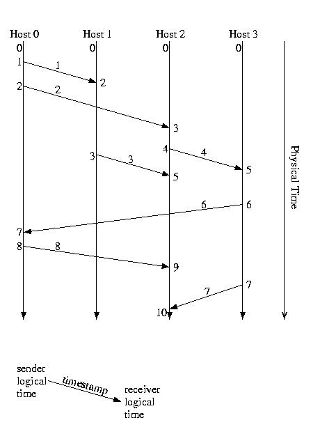
An Example of Lamport Logical Time
Causality and (Potential) Causality Violations
The example below shows several messages transmitted among the hosts of a distributed system. It is a simpler illustration of the systems' understanding of Lamport time and the timestamps placed onto each message.

Notice in the diagram above that the first message sent, from P0 to P1, is the last message received. Notice also that a message is sent from P0 to P2 and another from P2 to P3. The important thing about this situation is that the message from P2 arrives at P1, before the earlier message from P0. This timing problem might prove to be critical.
Let's put the messages above into a specific context, let's assume that an object migrated from P0 to P1, and ask ourselves what the figure might suggest:
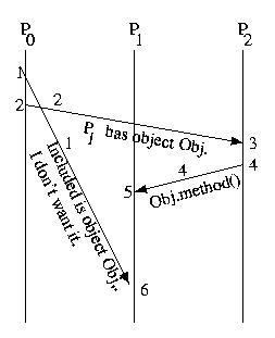
P0 gives Obj to P1 and tells P2. In response P2 sends a request to use that object to P1. Unfortunately, P1 has not yet received the message -- perhaps there was an error and the message needed to be resent or, perhaps, the communication channel is just slower. But, independent of the cause, "Bang!" P2's request to use the object fails.
This example illustrates a causality violation. A causality violation occurs when a message ordering problem results in one host taking an action based on information that another host has not yet, but should have, received. In this case P2 is trying to invoke a method on P1, because P2 thinks that P1 has Obj.
In designing systems, we assume that any action a host takes may be affected by any message it has previously received -- it requires application-specific knowledge to do otherwise. As a result, we would consider the situation above to be a potential causality violation, even if the message from P2 to P1 turned out to be completely independent of the messages that it received. Colloquially, we don't distinguish between potential causality violations and causality violations that have real consequences. Instead we call them both causality violations -- even if the messages turn out to be independent.
The bottom line is that a causality violation occurs if the send of a message knows something that the recipient of that message should know (has been sent), but does not know (has not received), by the time that the message is received.
Very shortly, we'll talk about designing a communication mechanism that avoid causality violations. But for the moment, lasts ask ourselves, "How can we detect (after the fact) that a causality violation has occurred?"
Lamport time is not sufficient to do this, because it track the total number of events in the system. This isn't helpful -- instead, we need a way of determining if messages were sent and received in the same order. In other words if we receive M2 before M1, but M1 was sent before M2, a (potential) causality violation has occured. The same is true if one or both of the messages arrived indirectly via other hosts. This is one of the areas where our next topic, vector time, becomes particularly useful.
Vector Logical Time
Vector logical time can be used to detect causality violations after-the fact. Let's discuss vector logical time -- and then take a look at how we can detect prior causality violations by comparing the current local time with the timestamp of an incoming message.As with Lamport logical time each host maintains its own notion of the local time and updates it using the timestamps placed by the sender onto messages. But with vector logical time, the time contains more information -- it contains a vector representing the state of each host. In other words, this vector not only contains the event count for the host, itself, it also contains the last-known event counts on each and every other host.
The only entry in this vector that is guaranteed to be up-to-date is the entry that represents the sender. For this reason, it is possible that the receiver may have a more up-to-date understanding of the logical time on some of the hosts. This would be the case if a message was sent from another host to the sender, but has not been received by the recipient.
As a result, when a hosts receives a message, it merges its time vector and the timestamp sent with the message -- it selects the higher of the values for each element. This ensures that the sender has information that is at least as up-to-date as the receiver.
Below is a summary of the rules for vector logical clocks:
- Instead of just keeping our logical time, we keep a vector, V[], such that V[i] represents what we know of the logical time on processor i.
- V[our_id] is our logical time
- Send V[] vector with each message
- On receive, merge both vectors, selecting the greater of the corresponding elements from each. Then increment the component for self. The event is said to have happened at new (incremented) time.
- On send, increment time component for self. Send the updated timestamp vector with the message. The event is said to have happened at new (incremented) time.
Recall this example from earlier:
Let's label it in vector time, just for practice:
Comparing Vector Timestamps
When comparing vector timestamps, we compare them by comparing each element in one timestamp to the corresponding element in the other timestamp.
- If corresponding elements in two timestamps are identical, the two events are the same event -- timestamps of different events should never be identical.
- If EventA "happens before" EventB then each element of EventA's timestamp is less than or equal to the corresponding element in EventB's timestamp, and at least one element is less than the corresponding element in EventB's timestamp.
- If EventB "happens before" EventA then each element of EventA's timestamp is greater than or equal to the corresponding element in EventB's timestamp, and at least one element is greater than the corresponding element in EventB's timestamp.
- If two events are concurrent, they will have "mixed" timestamps such that at least one pair of corresponding elements is "greater than" and at least one corresponding pair of elements is "less than."
The above definition of vector timestamp comparison ensures both of the following properties:
EventA "happens before" EventB ==> Vector_Timestamp (EventA) < Vector_Timestamp (EventB)Vector_Timestamp (EventA) < Vector_Timestamp (EventB) ==> EventA "happened before" EventB
Detecting Causality Violations Using Vector Timestamps
We can detect a causality violation using vector timestamps by comparing the timestamp of a newly received message to the local time. If the message's timestamp is less than the local time vector, a (potential) causality violation has occurred.Why? For the local time to have advanced such that it is ahead of the timestamp of the newly received message, a prior message must have advanced the local time. The sender of that prior message must have gotten the newly arrived message before it sent its prior message to us. Thus a (potential) causality violation occured.
Admittedly, this doesn't fix the problem -- but at least we have a way of detecting and logging the problem. This will make it much easier to isolate and debug or system -- or at least to take mitigating action to ensure that the output from the system is correct.
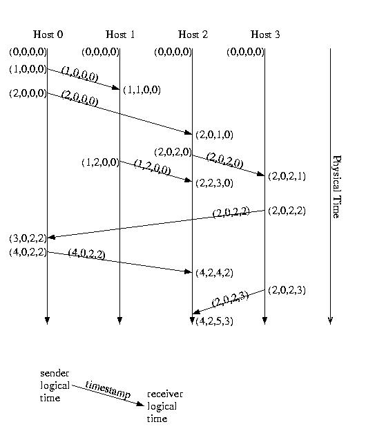
Now, let's consider the this familiar example again:
This time, let's label it using vector logical time and vector timestamps:

Notice that the timestamp on the M1 indicates a causality violation. M1's timestamp is (1,0,0). The local time on P2 is (2,0,2). (1,0,0) is less than (2,0,2). This indicates that a causality violation has occured -- someone who had already seen M1 sent P2 a message, before P2 received M1.
If the timestamps are concurrent, this does not represent a problem -- the messages are unrelated.
Matrix Logical Clocks
Before we leave time to discuss communication, let me mention one more detail. There is actually another type of logical clock that is one step more encompassing than a vector logical clock -- the matrix logical clock. Much like a vector clock maintains the simple logical time for each host, a matrix clock maintains a vector of the vector clocks for each host.Every time a message is exchanged, the sending host tells us not only what it knows about the global state of time, but what other hosts have told it that they know about the global state of time -- relaible gossip.
This is useful in applications such as checkpointing and recovery, and garbage collection. In these cases, having a lower bound on what another host knows can prove useful by enabling the disposal of unusable objects. In the case of garbage collection -- objects that are no other object can reference. In the case of recovery -- logs and/or checkpoints that are no longer needed.
We'll discuss matrix time in more detail when we discuss checkpointing and recovery -- it is much easier to understand with a clear application.