Game Trees

In this lecture we look at using trees for game playing, in particular the problems of searching game trees. We will classify all games into the folowing three groups

1. Single-player pathfinding problems.
   • Rubik’s Cube
   • Sliding puzzle.
   • Travelling Salesman Problem.
2. Two-player games.
   • Chess
   • Checkers
   • Othello
3. Constraint satisfaction problems.
   • Eight Queens
   • Sudoku

Each game consists of a problem space, an initial state, and a single (or a set of) goal states. A problem space is a mathematical abstraction in a form of a tree:

• the root represents current state
• nodes represent states of the game
• edges represent moves
• leaves represent final states (win, loss or draw)

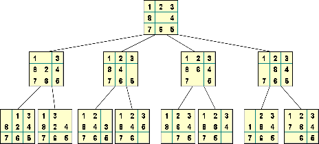
For example, in the 8-Puzzle game

• nodes: the different permutations of the tiles.
• edges: moving the blank tile up, down, right or left.

For some problems, the choice of a problem space is not so obvious. One general rule is that a smaller representation, in the sense of fewer states to search, is often better then a larger one. A problem space is characterized by two major factors.

How to search for a move?

Brute-Force Searches

• Breadth-First Search (BFS)

  BFS expands nodes in order of their depth from the root.

  Implemented by first-in first-out (FIFO) queue.

  BFS will find a shortest path to a goal.

  Time/Space Complexity - branching factor b and the solution depth d. Generate all the nodes up to level d.

  total number of nodes = 1 + b + b^2 + ... + b^d = O(b^d)
  

  BFS will exhaust the memory in minutes.

• Depth-First Search (DFS)

  Implemented by LIFO stack

  Space Complexity is linear in the maximum search depth.

  DFS generate the same set of nodes as BFS - Time Complexity is O(b^d)

  The first solution DFS found may not be the optimal one.

  On infinite tree DFS may not terminate.

• Depth-First Iterative-Deepening

  First performs a DFS to depth one. Than starts over executing DFS to depth two and so on

Minimax

We consider games with two players in which one person's gains are the result of another person's losses (so called zero-sum games). The minimax algorithm is a specialized search algorithm which returns the optimal sequence of moves for a player in an zero-sum game. In the game tree that results from the algorithm, each level represents a move by either of two players, say A- and B-player. Below is a game tree for the tic-tac-toe game

The minimax algorithm explores the entire game tree using a depth-first search. At each node in the tree where A-player has to move, A-player would like to play the move that maximizes the payoff. Thus, A-player will assign the maximum score amongst the children to the node where Max makes a move. Similarly, B-player will minimize the payoff to A-player. The maximum and minimum scores are taken at alternating levels of the tree, since A and B alternate turns.

The minimax algorithm computes the minimax decision for the leaves of the game tree and than backs up through the tree to give the final value to the current state.

Heuristic Search

So far we have looked at search algorithms that can in principle be used to systematically search the whole search space. Sometimes however it is not feasible to search the whole search space - it's just too big. In this case we need to use heuristic search. The basic idea of heuristic search is that, rather than trying all possible search paths, we focus on paths that seem to be getting us closer to the goal state. Of course, we generally can't be sure that we are really near the goal state, but we might be able to have a good guess. Heuristics are used to help us make that guess.

To use heuristic search we need an evaluation function that rankes nodes in the search tree according to some criteria (for example, how close we are to the target). This function provides a quick way of guessing.

Best First Search.
The search is similar to BFS, but instead of taking the first node it always chooses a node with the best score, according to an evaluation function. If we create a good evalution function, best first search may drastically cut down the amount of search time.

Here are the two most important properties of a heuristic function:

• it must provide an accurate estimator of the cost to reach a goal.
• it must be cheap to compute.
• it always must be a lower bound on actual solution cost.

A* algorithm
Best first search doesn't take into account the cost of the path from a start state to the current state. So, we may find a solution but it may be not a very good solution. There is a variant of best first search known as A* which attempts to find a solution which minimizes the total cost of the solution path. This algorithm combines advantages of breadth first search with advantages of best first search.

In the A* algorithm the score assigned to a node is a combination of the cost of the path so far A(S) and the estimated cost E(S) to solution.

H(S) = A(S) + E(S)