Spanning Trees

A Spanning Tree is a tree created from a graph that contains all of the nodes of the graph, but no cycles. In other words, you can create a minimum spanning tree from a graph, by removing one edge from any path that forms a cycle.

In the end, this will leave you with another graph, that is also a tree. If this graph contains N nodes, it will contain N-1 edges.

It contains at least N-1 edges, because this many are required to attach each node to the graph. Think of it this way. If the graph contains 1 node, there is nothing to attach it to -- as a result, no edges are needed. If we add nodes to the graph one at a time, we will need to use an edge to attach the new node to the graph. If we add a node, without adding an edge, we've really created a new graph with only one node -- we haven't expanded the old one, because we haven't established a relationship between the new node and any node in the old graph.

It contains at most N-1 edges, because more than one edge per node will create cycles, which would violate the definition of a tree. Imagine that you have a graph, any graph, with the minimum number, N-1, edges. Draw out your imaginary graph.

Now, try to add another edge to your graph, without creating a cycle. You can't do it. The reason is that each node, is already connected to another node of the graph. Adding an additional edge will connected it to a second point on the same graph. As a result, the graph will have a cycle -- it is no longer a tree.

Creating Spanning trees: Traversing Graphs

Today we are going to talk about two different ways of creating minimum spanning trees: the Depth-First Search and the Breadth-First Search. These algorithms are going to be very similar to the algorithms we studied for traversing trees.

The big difference is that we are going to mark the edges as we visit them, and avoid revisiting marked nodes. This is necessary, because graphs may have cycles -- and we don't want to go around-and-around ground we have already covered. So, if we leave a trail of breadcrumbs, and avoid recovering the ground we've already walked.

We can construct a spanning tree by keeping track of the path we follow to reach each node. In other words, we can start out with an empty graph, in addition to the one that we want to traverse. Then, instead of, or in addition to, printing each node we reach during the traversal, we can also add it to the new graph, by creating the same edge that we followed in the traversal to reach it.

So, if we get to Node-X from Node-Y, we then add an edge to Node-X from Node-Y in our new graph. Then, in the end, the new graph has the same nodes as the old graph -- but only one edge connecting each pair.

Depth First Search

Depth First Search (DFS) is a generalization of the preorder traversal. Starting at some arbitrarily chosen vertex v, we mark v so that we know we've visited it, process v, and then recursively traverse all unmarked vertices adjacent to v (v will be a different vertex with every new method call).

When we visit a vertex in which all of its neighbors have been visited, we return to its calling vertex, and visit one of its unvisited neighbors, repeating the recursion in the same manner. We continue until we have visited all of the starting vertex's neighbors, which means that we're done. The recursion (stack) guides us through the graph.

Performing a DFS on the following graph:

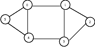
1. Any vertex can be the starting vertex. We choose to visit 1 first. (push 1)
2. From 1, we can go on to 0, 2, or 3.
3. We visit 0. (push 0) [0]
4. From 0, we can go on to 4 or 5 (we've already been to 1). We visit 4. (push 4) [4 0]
5. From 4, we can go on to 3 or 5 (we've already been to 0). We visit 3. (push 3) [3 4 0]
6. From 3, we can go on to 2 or 4 (we've already been to 1). We visit 2. (push 2) [2 3 4 0]
   
   
7. Now we've gone as far as we can go (from 2, we've already visited both 1 and 3). We can start returning.
   
   
8. We return to 3. (pop 2) [3 4 0]
9. We've already been to 1, 2, and 4, so we return.
10. We return to 4. (pop 3) [4 0]
    
    
11. We've already been to 0 and 3, but not to 5. We visit 5. (push 5) [5 4 0] (pop 5, pop 4, pop 0) []
    
    
12. We're done.

Pseudocode for DFS

public void depthFirstSearch(Vertex v)
{
	v.visited = true;
        // print the node or add it to the new spanning tree here
	for(each vertex w adjacent to v)
		if(!w.visited)
			depthFirstSearch(w);		
}

Breadth First Search

Breadth First Search (BFS) searches the graph one level (one edge away from the starting vertex) at a time. In this respect, it is very similar to the level order traversal that we discussed for trees.

Starting at some arbitrarily chosen vertex v, we mark v so that we know we've visited it, process v, and then visit and process all of v's neighbors.

Now that we've visited and processed all of v's neighbors, we need to visit and process all of v's neighbors neighbors. So we go to the first neighbor we visited and visit all of its neighbors, then the second neighbor we visited, and so on. We continue this process until we've visited all vertices in the graph. We don't use recursion in a BFS because we don't want to traverse recursively. We want to traverse one level at a time.

So imagine that you visit a vertex v, and then you visit all of v's neighbors w. Now you need to visit each w's neighbors. How are you going to remember all of your w's so that you can go back and visit their neighbors? You're already marked and processed all of the w's. How are you going to find each w's neighbors if you don't remember where the w's are? After all, you're not using recursion, so there's no stack to keep track of them.

To perform a BFS, we use a queue. Every time we visit vertex w's neighbors, we dequeue w and enqueue w's neighbors. In this way, we can keep track of which neighbors belong to which vertex. This is the same technique that we saw for the level-order traversal of a tree. The only new trick is that we need to makr the verticies, so we don't visit them more than once -- and this isn't even new, since this technique was used for the blobs problem during our discussion of recursion.

Performing a BFS on the same graph:

1. We choose to start by visiting 1. (enqueue 1) [1]
   
   
2. We visit 0, 2, and 3 because they are all one step away. (dequeue 1, enqueue 0, enqueue 2, enqueue 3) [0 2 3]
   
   
3. Because we visited 0 first, we go back to 0 and visit its neighbors, 4 and 5. (dequeue 0, enqueue 4, enqueue 5) [2 3 4 5] 2 and 3 have no unvisited neighbors. (dequeue 2, dequeue 3, dequeue 4, dequeue 5) [ ]
   
   
4. We're done.

Pseudocode

public void breadthFirstSearch(vertex v)
{
	Queue q = new Queue();
	
	v.visited = true;
	q.enQueue(v);
	
	while( !q.isEmpty() )
	{
  		Vertex w = (Vertex)q.deQueue();
                // Pritn the node or add it to the spanning tree here.
  		
		for(each vertex x adjacent to w)
		{			
			if( !x.visited )
			{
				x.visited = true;
				q.enQueue(x);
			}
		}
	}
}

Greedy Algorithms

Today we are going to study one algorithm for finding the shortest path between two verticies of a graph. It is known as Dijkstra's Algorithm. Dijkstra's algorithm is an example of a Greedy Algorithm. Greedy Algorithms operate by breaking a decision making process down into small steps, and making the best decision at each step. For many problems, this approach will lead to the best possible overall solution -- for others, it will not.

For example, we "make change", by using a greedy algorithm. We hand back $10 bills, until handing back another $10 would be giving back too much money. Then we hand out $5 bills, then $1 bills, then quarters, then dimes, then nickels, then pennies. In the end, we are guaranteed that we have returned the correct amount of change -- with the fewest possible bills or coins.

But, this algorithm would not work, for example, if we had 12-cent coins. Normally, if we have to return 21-cents of change, we return dime-dime-penny. But, with a 12-cent coin, let's call it the "dozen", we'd return dozen-nickel-penny-penny-penny-penny. From this example, we can see that greedy algorithms are appropriate for some problems -- but not all problems.

But, Dijkstra's Algorithm, is a greedy algorithm -- and does actually work. It is used to route packets throughout the Internet. Let's discover the magic:

Dijkstra's Algorithm: Shortest Path Algorithm for Weighted Graphs

One common use of graphs is to find the shortest path from one place to another. You may have at some point used an online program to find driving directions, and you likely had to specify if you wanted the shortest route/fastest route. This involves finding the shortest path in a weighted graph. The general algorithm to solve the shortest path problem is known as Dijkstra's Algorithm.

Dijskstra's createss, in successive steps, a spanning tree, rooted at the starting vertex. The resulting tree is rooted at this starting vertex To begin the root vertex v, is selected and it is added to the tree. At each stage, a vertex is added to the tree by choosing the vertex u such that the cost of getting from v to u is the smallest possible cost (the cost might, for example represent a distance in miles). At each stage, you ask thre question, "Where can I get from here?" and go down the shortest road possible from where you are.

Applying this algorithm until all vertices of the given graph are in the tree creates a spanning tree of that graph. And, this spanning tree has the interesting property that the path from the root to any node has the lowest possible total/aggegate weight.

Suppose we have the following graph:

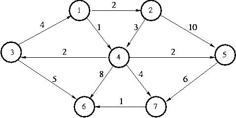
This graph is a directed graph, but it could just as easily be undirected.

Let's call the starting vertex s vertex 1. Just a reminder before we begin: the point of a shortest path algorithm is to find the shortest path to s from each of the other vertices in the graph.

The first vertex we select is 1, with a path of length 0. We mark vertex 1 as known.

	Known	Path	Length
1	Y	1	0
2	-	-	INF
3	-	-	INF
4	-	-	INF
5	-	-	INF
6	-	-	INF
7	-	-	INF

The vertices adjacent to 1 are 2 and 4. We adjust their fields.

	Known	Path	Length
1	Y	1	0
2	-	1	2
3	-	-	INF
4	-	1	1
5	-	-	INF
6	-	-	INF
7	-	-	INF

Next we select vertex 4 and mark it known. Vertices 3, 5, 6, and 7 are adjacent to 4, and we can improve each of their Length fields, so we do.

	Known	Path	Length
1	Y	1	0
2	-	1	2
3	-	4	3
4	Y	1	1
5	-	4	3
6	-	4	9
7	-	4	5

Next we select vertex 2 and mark it known. Vertex 4 is adjacent but already known, so we don't need to do anything to it. Vertex 5 is adjacent but not adjusted, because the cost of going through vertex 2 is 2 + 10 = 12 and a path of length 3 is already known.

	Known	Path	Length
1	Y	1	0
2	Y	1	2
3	-	4	3
4	Y	1	1
5	-	4	3
6	-	4	9
7	-	4	5

The next vertex we select is 5 and mark it known at cost 3. Vertex 7 is the only adjacent vertex, but we don't adjust it, because 3 + 6 > 5. Then we select vertex 3, and adjust the length for vertex 6 is down to 3 + 5 = 8.

	Known	Path	Length
1	Y	1	0
2	Y	1	2
3	Y	4	3
4	Y	1	1
5	Y	4	3
6	-	3	8
7	-	4	5

Next we select vertex 7 and mark it known. We adjust vertex 6 down to 5 + 1 = 6.

	Known	Path	Length
1	Y	1	0
2	Y	1	2
3	Y	4	3
4	Y	1	1
5	Y	4	3
6	-	7	6
7	Y	4	5

Finally, we select vertex 6 and make it known. Here's the final table.

	Known	Path	Length
1	Y	1	0
2	Y	1	2
3	Y	4	3
4	Y	1	1
5	Y	4	3
6	Y	7	6
7	Y	4	5

Now if we need to know how far away a vertex is from vertex 1, we can look it up in the table. We can also find the best route, for example, from the starting city (the one we selected as the route) to any other city (any other node). We just use the Path field to find the destinations predecessor, then use that node's path field to find its predecessor, and so on.

Shortest Path Algorithm for Unweighted Graphs

Unweighted graphs are a special case of weighted graphs. They can be addressed using Dijkstra's algorithm, as above -- just assume that all of the edges weigh the same thing, such as 1. Or, we can actually take a little bit of a shortcut.

For unweighted graphs, we don't actually need the "known" column of the table. This is because as soon as we discover a path to a vertex, we have discovered the best path -- there is no way we can find a better path. As a result, the verticies become "known" as soon as we find the first way to get there. We might subsequently find an equally good way -- but never a better way.

Let's think about the situation in Dijkstra's Algorithm that resulted in the discovery of a "better" path to a vertex that was already reachable. This situation occured, if a path with more "hops" was shorter than a path with fewer "hops". In other words, Dijkstra's algorithm reaches nodes in the same order as a breadth-first search -- reaching all nodes one hop from the start, then those two hops from the start, then those three hops from the start, and so on.

But, since not all of the hops are of the same length, one hop might be really long, for example it might have a cost of 100. But, another path between the same nodes, might involve three hops, of lengths, 10, 20, and 30. It is cheaper to go the three hops 10+20+30=60 than the single hop of 100. Yet, the hop of 100 is the path that is discovered first. As a result, we need to check subsequent paths that pass through more verticies, until we are sure that we can't find a better path, at which time, we finally mark the node (and the path to it) as known.

Since, in an unweighted graph, all of the edges are modeled as having the same weight, it is impossible for this situation to occur. Two hops will always be longer than three hops, &c.

Since the algorithm is proceeding in a depth-first fashion, we find things that are one hop away before things that are two hops away, before things that are three hops away, and so on. As a result, in an unweighted graph, as soon as we find a node, it is known -- there can be no better way of finding it.

Let's consider an example for the graph shown below.

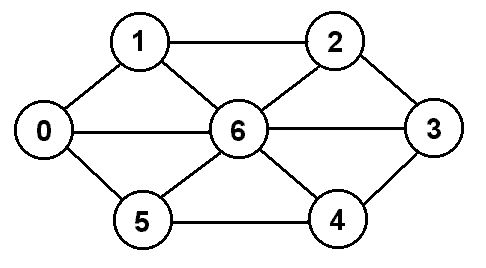
We would build a table as follows:

	Known	Path	Length
0	-	-	INF
1	-	-	INF
2	-	-	INF
3	-	-	INF
4	-	-	INF
5	-	-	INF
6	-	-	INF

In the table, the index on the left represents the vertex we are going to (for convenience, we will assume that we are starting at vertex 0). This time, we will ignore the Known field, since it is only necessary if the edges are weighted. The Path field tells us which vertex precedes us in the path. The Length field is the length of the path from the starting vertex to that vertex, which we initialize to INFinity under the assumption that there is no path unless we find one, in which case the length will be less than infinity.

We begin by indicating that 0 can reach itself with a path of length 0. This is better than infinity, so we replace INF with 0 in the Length column, and we also place a 0 in the Path column. Now we look at 0's neighbors. All three of 0's neighbors 1, 5, and 6  can be reached from 0 with a path of length 1 (1 + the length of the path to 0, which is 0), and for all three of them this is better, so we update their Path and Length fields, and then enqueue them, because we will have to look at their neighbors next.

We dequeue 1, and look at its neighbors 0, 2, and 6. The path through vertex 1 to each of those vertices would have a length of 2 (1 + the length of the path to 1, which is 1). For 0 and 6, this is worse than what is already in their Length field, so we will do nothing for them. For 2, the path of length 2 is better than infinity, so we will put 2 in its Length field and 1 in its Path field, since it came from 1, and then we will enqueue so we can eventually look at its neighbors if necessary.

We dequeue the 5 and look at its neighbors 0, 4, and 6. The path through vertex 5 to each of those vertices would have a length of 2 (1 + the length of the path to 5, which is 1). For 0 and 6, this is worse than what is already in their Length field, so we will do nothing for them. For 4, the path of length 2 is better than infinity, so we will put 2 in its Length field and 5 in its Path field, since it came from 5, and then we will enqueue it so we can eventually look at its neighbors if necessary.

Next we dequeue the 6, which shares an edge with each of the other six vertices. The path through 6 to any of these vertices would have a length of 2, but only vertex 3 currently has a higher Length (infinity), so we will update 3's fields and enqueue it.

Of the remaining items in the queue, the path through them to their neighbors will all have a length of 3, since they all have a length of 2, which will be worse than the values that are already in the Length fields of all the vertices, so we will not make any more changes to the table. The result is the following table:

	Known	Path	Length
0	-	0	0
1	-	0	1
2	-	1	2
3	-	6	2
4	-	5	2
5	-	0	1
6	-	0	1

Now if we need to know how far away a vertex is from vertex 0, we can look it up in the table, just as before. And, just as before, we can use the path field to discover the rout from the starting node to any vertex.