Kruskal's Algorithm

last class, we discussed Prim's Algorithm for finding a minimum spanning tree. Today, we are going to discuss a second appraoch for solving the same problem. This approach is also a greedy algorithm.

Althoguh the implementation is a bit more comples, the basic algorithm is very straight-forward. We simple attempt to add each edge from the original graph to the minimum spanning tree, beginning with the lowest-weight edge and finishing with the greatest-weight edge. We add the edge if it doesn't cause a cycle and passs it up, if it does. We continue to add edges, until we've added N-1 edges, where N is the number of verticies. Remember, spanning trees have exactly N-1 edges -- never more, never less.

In order to make it easy to select the candidates in the right order, from the lowest weight to the highest weight, we store the edges in a priority queue (heap). Then, selecting an edge is simply the deleteMin() operation.

Another way of viewing the algorithm is to views the inital configuration as a forrest of trees, with each vertex in its own, independent tree. If we take this view, then adding an edge merges two trees into one. When Kruskal's terminates, there is only one tree - the minimum spanning tree.

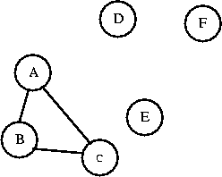
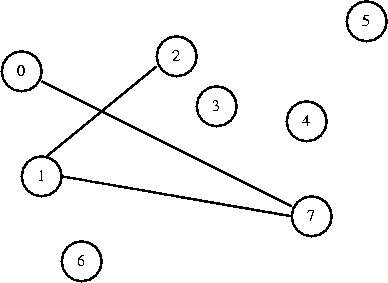
Let's take a look at the algorithm in operation, using the smae graph as we used last class:

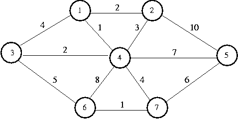
The following table shows the verticies sorted by weight and whetehr or not each vertex was accepted. Remember, we evaluate each vertex, one-at-a-time, from the top of this list down. In a real implemention, we would have added them to a heap, and be using deleteMin() to get to the top one for each iteration.

Edge	Weight	Action
(1,4)	1	Accepted
(6,7)	1	Accepted
(1,2)	2	Accepted
(3,4)	2	Accepted
(2,4)	3	Rejected
(1,3)	4	Rejected
(4,7)	4	Accepted
(3,6)	5	Rejected
(5,7)	6	Accepted

Using Sets to Detect Cycles

So, how can we figure out if adding a particular edge to a tree will create a cycle? This is very important to Kruskal's Algorithm, because we only add an edge, if doing so won't create a cycle.

Imagine that each vertex in a graph is its own set (remember the Set class you created for the lab?).

If you connect two vertices in the same set together, you'll create a cycle. As long as you connect vertices from two different sets, you won't create a cycle. A and B are in different sets. I'll connect them.

Now AB is a set. Can I connect C to AB? C and AB are in different sets, I'll connect them. Now I have a set called ABC.

Can I connect C to B? C and B are in the same set, so connecting them will create a cycle.

Union-Find

Earlier this semester, we created a Set class using LinkedLists. This class supported a very broad array of Set operations. But, for this particular problem, we only need to do two things: look in a set to see if an item is there (find) and unite two sets (union). And, since the Set lab, we've learned about trees, which added a powerful tool to our kit. Let's see how we can use trees to represent sets in a way that leads to efficient Union and Find operations.

Again, imagine a graph, with each vertex as its own set. Now imagine that each set of vertices is a tree. So before we connect any edges, each vertex is its own tree, and the graph is a forest of trees.

We'll use an array to represent the trees. Create an array, with each index of the array representing the corresponding vertex of the graph. Place a sentinel value, -1, into each array element. We will use this sentinel value to denote the root of the tree. Before we connect any edges, each vertex is its own tree, so its the root. -1 represents the root of the tree set.

  0    1    2    3    4    5    6    7
  [-1] [-1] [-1] [-1] [-1] [-1] [-1] [-1]
  

Now I decide to connect 7 to 1. They are in different sets, so I connect them.

  0    1    2    3    4    5    6    7
  [-1] [-1] [-1] [-1] [-1] [-1] [-1] [ 1]
  

The parent of 7 is now 1, and 7 is no longer the root of the tree. If we want to find 7's parent, we simply look at its value, which is 1. To find 1's parent, we look at its value, which is -1, indicating that 1 has no parent and is the root of the tree.

Now I decide to connect 2 to 1. They are in different sets, so I connect them.

  0    1    2    3    4    5    6    7
  [-1] [-1] [ 1] [-1] [-1] [-1] [-1] [ 1]
  

Now I decide to connect 0 to 7. They are in different sets, so I connect them.

  0    1    2    3    4    5    6    7
  [ 7] [-1] [ 1] [-1] [-1] [-1] [-1] [ 1]
  

I want to connect 4 to 6. They are in different sets, so I connect them.

  0    1    2    3    4    5    6    7
  [ 7] [-1] [ 1] [-1] [ 6] [-1] [-1] [ 1]
  

I want to connect 5 to 6. They are in different sets, so I connect them.

  0    1    2    3    4    5    6    7
  [ 7] [-1] [ 1] [-1] [ 6] [ 6] [-1] [ 1]
  

Note that connect 4 to 5 would now create a cycle.

I want to connect 1 to 4. They are in different sets, so I connect them.

  0    1    2    3    4    5    6    7
  [ 7] [ 4] [ 1] [-1] [ 6] [ 6] [-1] [ 1]
  

How do you find out what set a particular vertex of the graph belongs to? You simply follow its ancestors up until you find an array element with a value of -1. At this point, all vertices except 3 are in the same set -- 6. 6 is the only element with a value of -1. Vertex 6 is the root of the tree consisting of all of the vertices in the graph.

The operation that connects to vertices by changing the array element value of one to be the other is called union. The operation that finds the root of a particular vertex's tree is called find.

Dijkstra's Algorithm: Shortest Path Algorithm for Weighted Graphs

One common use of graphs is to find the shortest path from one place to another. You may have at some point used an online program to find driving directions, and you likely had to specify if you wanted the shortest route/fastest route. This involves finding the shortest path in a weighted graph.

The general algorithm to solve the shortest path problem is known as Dijkstra's Algorithm. Dijkstra's algorithm proceeds in stages using an approach and a table very similar to the one we used last class for Prim's Algorithm. The big difference is that the "cost function" changes.

With Prim's algorithm, the edge that we wanted to add to the tree was the edge closest to any other edge already in the tree. In the example of the electrician, this was the electrical outlet that would requires the shortest piece of wire to reach any other outlet in the circuit.

With Dijkstra's algorithm, we aren't concered about reaching any other point, we are concerned about reaching the starting point. So, we care about the total distance from start-to-finish, instead fo the distance from one vertex to another. As a result the column of the table that keeps track of the cost/weight/length for a particula vertex keeps track of the total distance from start to that vertex, not just the distance to the prior vertex in the path. So, we compute the total distance by adding the next leg of the trip to the total of all prior legs. Then, we compare this to the best total we have found so far, and replace it, if we;ve found a better route.

With the exception of the change to the cost function, the algorithm remains entirely unchanged. We're just coptimizing for the shortest distance from the start (root of the tree) instead of the shortest distance to the prior vertex.

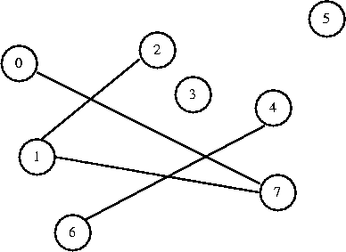
Suppose we have the following graph:

This graph is a directed graph, but it could just as easily be undirected.

Let's call the starting vertex s vertex 1. Just a reminder before we begin: the point of a shortest path algorithm is to find the shortest path to s from each of the other vertices in the graph.

The first vertex we select is 1, with a path of length 0. We mark vertex 1 as known.

	Known	Path	Length
1	Y	1	0
2	-	-	INF
3	-	-	INF
4	-	-	INF
5	-	-	INF
6	-	-	INF
7	-	-	INF

The vertices adjacent to 1 are 2 and 4. We adjust their fields.

	Known	Path	Length
1	Y	1	0
2	-	1	2
3	-	-	INF
4	-	1	1
5	-	-	INF
6	-	-	INF
7	-	-	INF

Next we select vertex 4 and mark it known. Vertices 3, 5, 6, and 7 are adjacent to 4, and we can improve each of their Length fields, so we do.

	Known	Path	Length
1	Y	1	0
2	-	1	2
3	-	4	3
4	Y	1	1
5	-	4	3
6	-	4	9
7	-	4	5

Next we select vertex 2 and mark it known. Vertex 4 is adjacent but already known, so we don't need to do anything to it. Vertex 5 is adjacent but not adjusted, because the cost of going through vertex 2 is 2 + 10 = 12 and a path of length 3 is already known.

	Known	Path	Length
1	Y	1	0
2	Y	1	2
3	-	4	3
4	Y	1	1
5	-	4	3
6	-	4	9
7	-	4	5

The next vertex we select is 5 and mark it known at cost 3. Vertex 7 is the only adjacent vertex, but we don't adjust it, because 3 + 6 > 5. Then we select vertex 3, and adjust the length for vertex 6 is down to 3 + 5 = 8.

	Known	Path	Length
1	Y	1	0
2	Y	1	2
3	Y	4	3
4	Y	1	1
5	Y	4	3
6	-	3	8
7	-	4	5

Next we select vertex 7 and mark it known. We adjust vertex 6 down to 5 + 1 = 6.

	Known	Path	Length
1	Y	1	0
2	Y	1	2
3	Y	4	3
4	Y	1	1
5	Y	4	3
6	-	7	6
7	Y	4	5

Finally, we select vertex 6 and make it known. Here's the final table.

	Known	Path	Length
1	Y	1	0
2	Y	1	2
3	Y	4	3
4	Y	1	1
5	Y	4	3
6	Y	7	6
7	Y	4	5

Now if we need to know how far away a vertex is from vertex 1, we can look it up in the table. We can also find the best route, for example, from the starting city (the one we selected as the route) to any other city (any other node). We just use the Path field to find the destinations predecessor, then use that node's path field to find its predecessor, and so on.

Shortest Path Algorithm for Unweighted Graphs

Unweighted graphs are a special case of weighted graphs. They can be addressed using Dijkstra's algorithm, as above -- just assume that all of the edges weigh the same thing, such as 1. Or, we can actually take a little bit of a shortcut.

For unweighted graphs, we don't actually need the "known" column of the table. This is because as soon as we discover a path to a vertex, we have discovered the best path -- there is no way we can find a better path. As a result, the verticies become "known" as soon as we find the first way to get there. We might subsequently find an equally good way -- but never a better way.

Let's think about the situation in Dijkstra's Algorithm that resulted in the discovery of a "better" path to a vertex that was already reachable. This situation occured, if a path with more "hops" was shorter than a path with fewer "hops". In other words, Dijkstra's algorithm reaches nodes in the same order as a breadth-first search -- reaching all nodes one hop from the start, then those two hops from the start, then those three hops from the start, and so on.

But, since not all of the hops are of the same length, one hop might be really long, for example it might have a cost of 100. But, another path between the same nodes, might involve three hops, of lengths, 10, 20, and 30. It is cheaper to go the three hops 10+20+30=60 than the single hop of 100. Yet, the hop of 100 is the path that is discovered first. As a result, we need to check subsequent paths that pass through more verticies, until we are sure that we can't find a better path, at which time, we finally mark the node (and the path to it) as known.

Since, in an unweighted graph, all of the edges are modeled as having the same weight, it is impossible for this situation to occur. Two hops will always be longer than three hops, &c.

Since the algorithm is proceeding in a depth-first fashion, we find things that are one hop away before things that are two hops away, before things that are three hops away, and so on. As a result, in an unweighted graph, as soon as we find a node, it is known -- there can be no better way of finding it.

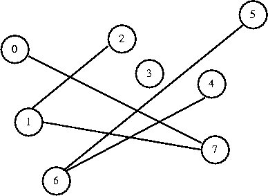
Let's consider an example for the graph shown below.

We would build a table as follows:

	Known	Path	Length
0	-	-	INF
1	-	-	INF
2	-	-	INF
3	-	-	INF
4	-	-	INF
5	-	-	INF
6	-	-	INF

In the table, the index on the left represents the vertex we are going to (for convenience, we will assume that we are starting at vertex 0). This time, we will ignore the Known field, since it is only necessary if the edges are weighted. The Path field tells us which vertex precedes us in the path. The Length field is the length of the path from the starting vertex to that vertex, which we initialize to INFinity under the assumption that there is no path unless we find one, in which case the length will be less than infinity.

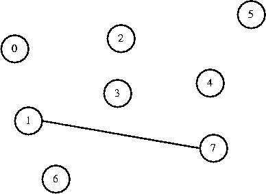
We begin by indicating that 0 can reach itself with a path of length 0. This is better than infinity, so we replace INF with 0 in the Length column, and we also place a 0 in the Path column. Now we look at 0's neighbors. All three of 0's neighbors 1, 5, and 6  can be reached from 0 with a path of length 1 (1 + the length of the path to 0, which is 0), and for all three of them this is better, so we update their Path and Length fields, and then enqueue them, because we will have to look at their neighbors next.

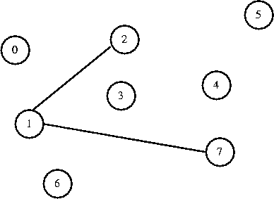
We dequeue 1, and look at its neighbors 0, 2, and 6. The path through vertex 1 to each of those vertices would have a length of 2 (1 + the length of the path to 1, which is 1). For 0 and 6, this is worse than what is already in their Length field, so we will do nothing for them. For 2, the path of length 2 is better than infinity, so we will put 2 in its Length field and 1 in its Path field, since it came from 1, and then we will enqueue so we can eventually look at its neighbors if necessary.

We dequeue the 5 and look at its neighbors 0, 4, and 6. The path through vertex 5 to each of those vertices would have a length of 2 (1 + the length of the path to 5, which is 1). For 0 and 6, this is worse than what is already in their Length field, so we will do nothing for them. For 4, the path of length 2 is better than infinity, so we will put 2 in its Length field and 5 in its Path field, since it came from 5, and then we will enqueue it so we can eventually look at its neighbors if necessary.

Next we dequeue the 6, which shares an edge with each of the other six vertices. The path through 6 to any of these vertices would have a length of 2, but only vertex 3 currently has a higher Length (infinity), so we will update 3's fields and enqueue it.

Of the remaining items in the queue, the path through them to their neighbors will all have a length of 3, since they all have a length of 2, which will be worse than the values that are already in the Length fields of all the vertices, so we will not make any more changes to the table. The result is the following table:

	Known	Path	Length
0	-	0	0
1	-	0	1
2	-	1	2
3	-	6	2
4	-	5	2
5	-	0	1
6	-	0	1

Now if we need to know how far away a vertex is from vertex 0, we can look it up in the table, just as before. And, just as before, we can use the path field to discover the rout from the starting node to any vertex.