Spanning Trees

A Spanning Tree is a tree created from a graph that contains all of the nodes of the graph, but no cycles. In other words, you can create a minimum spanning tree from a graph, by removing one edge from any path that forms a cycle.

In the end, this will leave you with another graph, that is also a tree. If this graph contains N nodes, it will contain N-1 edges.

It contains at least N-1 edges, because this many are required to attach each node to the graph. Think of it this way. If the graph contains 1 node, there is nothing to attach it to -- as a result, no edges are needed. If we add nodes to the graph one at a time, we will need to use an edge to attach the new node to the graph. If we add a node, without adding an edge, we've really created a new graph with only one node -- we haven't expanded the old one, because we haven't established a relationship between the new node and any node in the old graph.

It contains at most N-1 edges, because more than one edge per node will create cycles, which would violate the definition of a tree. Imagine that you have a graph, any graph, with the minimum number, N-1, edges. Draw out your imaginary graph.

Now, try to add another edge to your graph, without creating a cycle. You can't do it. The reason is that each node, is already connected to another node of the graph. Adding an additional edge will connected it to a second point on the same graph. As a result, the graph will have a cycle -- it is no longer a tree.

Creating Spanning trees: Traversing Graphs

Today we are going to talk about two different ways of creating minimum spanning trees: the Depth-First Search and the Breadth-First Search. These algorithms are going to be very similar to the algorithms we studied for traversing trees.

The big difference is that we are going to mark the edges as we visit them, and avoid revisiting marked nodes. This is necessary, because graphs may have cycles -- and we don't want to go around-and-around ground we have already covered. So, if we leave a trail of breadcrumbs, and avoid recovering the ground we've already walked.

We can construct a spanning tree by keeping track of the path we follow to reach each node. In other words, we can start out with an empty graph, in addition to the one that we want to traverse. Then, instead of, or in addition to, printing each node we reach during the traversal, we can also add it to the new graph, by creating the same edge that we followed in the traversal to reach it.

So, if we get to Node-X from Node-Y, we then add an edge to Node-X from Node-Y in our new graph. Then, in the end, the new graph has the same nodes as the old graph -- but only one edge connecting each pair.

Depth First Search

Depth First Search (DFS) is a generalization of the preorder traversal. Starting at some arbitrarily chosen vertex v, we mark v so that we know we've visited it, process v, and then recursively traverse all unmarked vertices adjacent to v (v will be a different vertex with every new method call).

When we visit a vertex in which all of its neighbors have been visited, we return to its calling vertex, and visit one of its unvisited neighbors, repeating the recursion in the same manner. We continue until we have visited all of the starting vertex's neighbors, which means that we're done. The recursion (stack) guides us through the graph.

Performing a DFS on the following graph:

1. Any vertex can be the starting vertex. We choose to visit 1 first. (push 1)
2. From 1, we can go on to 0, 2, or 3.
3. We visit 0. (push 0) [0]
4. From 0, we can go on to 4 or 5 (we've already been to 1). We visit 4. (push 4) [4 0]
5. From 4, we can go on to 3 or 5 (we've already been to 0). We visit 3. (push 3) [3 4 0]
6. From 3, we can go on to 2 or 4 (we've already been to 1). We visit 2. (push 2) [2 3 4 0]
   
   
7. Now we've gone as far as we can go (from 2, we've already visited both 1 and 3). We can start returning.
   
   
8. We return to 3. (pop 2) [3 4 0]
9. We've already been to 1, 2, and 4, so we return.
10. We return to 4. (pop 3) [4 0]
    
    
11. We've already been to 0 and 3, but not to 5. We visit 5. (push 5) [5 4 0] (pop 5, pop 4, pop 0) []
    
    
12. We're done.

Pseudocode for DFS

public void depthFirstSearch(Vertex v)
{
	v.visited = true;
        // print the node or add it to the new spanning tree here
	for(each vertex w adjacent to v)
		if(!w.visited)
			depthFirstSearch(w);		
}

Breadth First Search

Breadth First Search (BFS) searches the graph one level (one edge away from the starting vertex) at a time. In this respect, it is very similar to the level order traversal that we discussed for trees.

Starting at some arbitrarily chosen vertex v, we mark v so that we know we've visited it, process v, and then visit and process all of v's neighbors.

Now that we've visited and processed all of v's neighbors, we need to visit and process all of v's neighbors neighbors. So we go to the first neighbor we visited and visit all of its neighbors, then the second neighbor we visited, and so on. We continue this process until we've visited all vertices in the graph. We don't use recursion in a BFS because we don't want to traverse recursively. We want to traverse one level at a time.

So imagine that you visit a vertex v, and then you visit all of v's neighbors w. Now you need to visit each w's neighbors. How are you going to remember all of your w's so that you can go back and visit their neighbors? You're already marked and processed all of the w's. How are you going to find each w's neighbors if you don't remember where the w's are? After all, you're not using recursion, so there's no stack to keep track of them.

To perform a BFS, we use a queue. Every time we visit vertex w's neighbors, we dequeue w and enqueue w's neighbors. In this way, we can keep track of which neighbors belong to which vertex. This is the same technique that we saw for the level-order traversal of a tree. The only new trick is that we need to makr the verticies, so we don't visit them more than once -- and this isn't even new, since this technique was used for the blobs problem during our discussion of recursion.

Performing a BFS on the same graph:

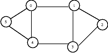
1. We choose to start by visiting 1. (enqueue 1) [1]
   
   
2. We visit 0, 2, and 3 because they are all one step away. (dequeue 1, enqueue 0, enqueue 2, enqueue 3) [0 2 3]
   
   
3. Because we visited 0 first, we go back to 0 and visit its neighbors, 4 and 5. (dequeue 0, enqueue 4, enqueue 5) [2 3 4 5] 2 and 3 have no unvisited neighbors. (dequeue 2, dequeue 3, dequeue 4, dequeue 5) [ ]
   
   
4. We're done.

Pseudocode

public void breadthFirstSearch(vertex v)
{
	Queue q = new Queue();
	
	v.visited = true;
	q.enQueue(v);
	
	while( !q.isEmpty() )
	{
  		Vertex w = (Vertex)q.deQueue();
                // Pritn the node or add it to the spanning tree here.
  		
		for(each vertex x adjacent to w)
		{			
			if( !x.visited )
			{
				x.visited = true;
				q.enQueue(x);
			}
		}
	}
}

Finding a Minimum Spanning Tree of an Undirected, Connected Graph

A minimum spanning tree of an undirected graph is a tree formed from that graph's edges that connects all the vertices of that graph at the lowest total cost. You can make a spanning tree of a graph only if the graph is connected. There may be more than one spanning tree of a particular graph.

The number of edges in a minimum spanning tree of a graph will be the number of vertices it has - 1. A minimum spanning tree is a tree because it's acyclic. It's spanning because it reaches every vertex in the graph, and it's minimum for the obvious reason. If we need to wire a house with a minimum of cable, then a we need to find a minimum spanning tree of a graph of the electrical layout of the house.

Minimum Spanning Trees: Why Do We Care?

Many real situations can be modeled with graphs. And, many real situations can be solved by finding the minimum spanning tree of graphs.

My favorite example involves an electrician and a house. Imagine that a collection of electrical outlets have been installed in the walls of a house, and that the electicity enters the house at a single electrical box. We can model this situation as a graph, where each of the outlets and the electrical box is a node, and the walls are the edges. The length of each wall, or segment thereof, is the distance along the wall between two of the electrical connections.

As a result, the electrician may have many different routes he can use to wire the outlets -- they may be reachable by different paths along the walls. So, the electrician wants to find the path that requires the least amount of wire. This saves money, becuase less wire is needed. And, it saves time, because the runs along the wal are shorter and, as a consequence, take less time to install.

To solve this problem, the electrician can model the outlets and wall segments conecting them as a graph rooted at the electrical box. Then, the electrician can find the minimum spanning tree of the graph. The edges in this tree give the paths that the electrician should use to run the wires -- they will reach each node, while requiring the least amount of wire.

Greedy Algorithms

Today we are going to study one algorithm for finding the minimum spanning tree of a graph. It is known as Prim's Algorithm. Prim's algorithm is an example of a Greedy Algorithm. Greedy Algorithms operate by breaking a decision making process down into small steps, and making the best decision at each step. For many problems, this approach will lead to the best possible overall solution -- for others, it will not.

For example, we "make change", by using a greedy algorithm. We hand back $10 bills, until handing back another $10 would be giving back too much money. Then we hand out $5 bills, then $1 bills, then quarters, then dimes, then nickels, then pennies. In the end, we are guaranteed that we have returned the correct amount of change -- with the fewest possible bills or coins.

But, this algorithm would not work, for example, if we had 12-cent coins. Normall, if we have to return 21-cents of change, we return dime-dime-penny. But, with a 12-cent coin, let's call it the "dozen", we'd return dozen-nickel-penny-penny-penny-penny. From this example, we can see that greedy algorithms are appropriate for some problems -- but not all problems.

But, Prim's Algorithm, is a greedy algorithm -- and does actually work. Let's take a look at a different example, the sidewalk example, and see how.

Prim's Algorithm

Imagine finding the minimum amount of sidewalk needed to get to every point of interest from the entrance of a park. Now think of the park entrance as the root of your minimum spanning tree. This will help you as you apply Prim's Algorithm.

Prim's grows the tree in successive stages. You start by choosing one vertex to be the root v, and add an edge (piece of sidewalk), and thus an associated vertex (a point of interest in the park), to the tree. At each stage, you add a vertex to the tree by choosing the vertex u such that the cost of getting from v to u is the smallest possible cost (in the case of the park, the cost is distance). At each stage, you say, "Where can I get from here?" and go down the shortest road possible from where you are.

Applying this algorithm until all vertices of the given graph are in the tree creates a minimum spanning tree of that graph.

Prim's finds the minimum spanning tree of the entire graph from s, so we use the Length field to record the cost of getting from a vertex v to its parent in the minimum spanning tree we're making.

Suppose we have the following graph:

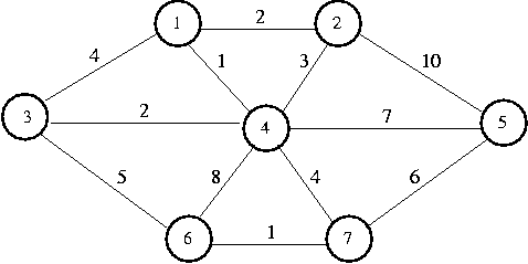
We would build a table as follows:

	Known	Path	Length
1	-	-	INF
2	-	-	INF
3	-	-	INF
4	-	-	INF
5	-	-	INF
6	-	-	INF
7	-	-	INF

Selecting vertex 1 and making it the root of our tree, we update its neighbors, 1, 2, 3, and 4. Vertex 1's cheapest place in the tree is known.

	Known	Path	Length
1	Y	1	0
2	-	1	2
3	-	1	4
4	-	1	1
5	-	-	INF
6	-	-	INF
7	-	-	INF

Next we select vertex 4 (one of the neighbors of vertex 1). It's cheapest place in the tree is now known. Every vertex in the graph is adjacent to 4.

Vertex 1 is known (meaning that its in its optimal place in the tree), so we don't examine it. We don't change vertex 2, because its Length is 2, and the edge cost from 4 to 2 is 3. We update the rest.

	Known	Path	Length
1	Y	1	0
2	-	1	2
3	-	4	2
4	Y	1	1
5	-	4	7
6	-	4	8
7	-	4	4

Next we select vertex 2 (another neighbor of 1) and make it known. We can't improve our tree in any way by going through vertex 2. We select vertex 3 (the last neighbor of 1) and make it known. The path from 3 to 6 is cheaper than the path from 4 to 6, so we update 6's fields.

2 and 3's cheapest places in the tree are now known.

	Known	Path	Length
1	Y	1	0
2	Y	1	2
3	Y	4	2
4	Y	1	1
5	-	4	7
6	-	3	5
7	-	4	4

Next we select vertex 7 (neighbor of 4, the first chosen neighbor of 1). Its cheapest place in the tree is now known. Now we can adjust vertices 5 and 6. Selecting 5 and 6 doesn't provide any cheaper paths. After 5 and 6 are selected, the Prim's algorithm terminates.

	Known	Path	Length
1	Y	1	0
2	Y	1	2
3	Y	4	2
4	Y	1	1
5	Y	7	6
6	Y	7	1
7	Y	4	4

To find the minimum spanning tree of the graph featured in the table, follow the Path fields from vertex 1.