Mastery Exam Overview

Today we're just going to walk through the pool of linked list and binary tree questions.

We're now in LL#1 pool, which is the easier of the two.

insertItemAfter - You want to create an index, start it at head, and then stop it when it equals null or the item you're finding. If it's null, then you can't insert anywhere so you just return, and if it's not then you insert it after that node.

insertItemBefore - This is a little more trickier, because if you just search for the item then you can't go back and insert it before. So you have to look one ahead of you. The only real trick is that you need a special case for the head, where the item to insert becomes the new head.

removeAllGreaterItems - If you're removing, then you need to look one ahead to remove it from the linked list. The head is a special case, and you should probably just take care of it last, because if the first 5 elements are all greater, then you'll have to remove the head 5 times. By just treating the head as a separate case you remove all the others except it, and then remove the head last if you need to.

removeAllLesserItems - Same as removeGreater except you compare for lesser.

removeFirstMatchingItem - No tricks here, except you need to look one ahead to remove, except for the special case of the head.

swapFirstAndLast - First, if it's empty or only one item just exit the method. If it has two items, then your head.getNext() is the tail, which is hard to set up for a general case, so treat that as a special case also. Otherwise, find a reference to one before the tail. Set the tail to the head, then the head to the tail, and take care of all the setNexts to make everything point the right way.

The LL#2 pool is probably the most time intensive of them. Many of the BST questions can be solved very quickly with recursion, but the LL#2 ones many times you just need to do brute-force. For a lot of these, a helper method that just tries to find an element in a linked list would be very helpful.

getItemsNotPresent - Walk through each item in the first array. If it's not in the second array add it to the list to return.

intersection - Walk through first list, try to find it in the second. If it's in the second, add to list to return

isPermutation - Simple way, walk through list 1 and look for each in list 2, and walk through list 2 and look for each in list 1. If you find anything not there, then return false, if you check every element in both and find them, return true.

isSubset - Same as isPermutation except you only have to check to make sure everything in list 1 is in list 2.

isSymmetric - Create a new list by walking through the original list and doing addHead() for each one. This would create a reversed list. Take two indices, and then walk through each item and compare each. If any are different, return false. If get to end of list, return true.

rotate - Find the size of the list, take the number of times to rotate, mod the size of the list, so if you have to rotate 15 times, you only really need to rotate 5 times for a 10 item list. Then just add head to tail or add tail to head that many times depending on if positive or negative.

shiftItemTowardsHead - If we want to shift towards the head, we want to have a count of how far from the head the item to shift is. If it's less than the number given, it says not to do anything so you're done. Otherwise, remove it from the list, and then add it at the place it needs to be.

shiftItemTowardsTail - Find the tail and walk past it to make sure there are enough nodes for it. If it is, then find the right place to swap, and swap them.

xOr - Walk through list 1, for each element if it isn't in list 2 then add it to the end. For items in list 2, do the same.

BST pool #1 is very easy if you know much about BSTs.

cloneTree - Make sure you insert in the same place. So the root of the cloned tree should be the same as the root of the original, etc. If you do a preorder traversal on the BST and then perform the insert, then you should get the same. Another way to do this is to copy the current node, and recursively call the cloneTree on the left and right subtrees.

maxLeafLevel - Recursively traverse the tree, each time you call yourself, add 1. When you get to the end, return your level. When you get them back, return the highest of the left and right.

minLeafLevel - Same as max, except return the min of left and right

numberOfInteriorNodes - If you are a leaf, return 0. If not, return the sum of 1 plus the recursive call to the left and right

numberOfLeaves - Count leaves in left and count leaves and right. Add the result of the two and return it if it is not a leaf, if it is then return 1.

printPath - This is essentially a BST search, so you want to just go left if it's less, go right if it's greater, and stop if it's equal. For every node you visit, the first thing you do is print the node you're at.

BST #2

balancedFactor - Return maxLeafLevel on left and right of the rootValue and return its difference.

getUniqueItems - You don't need to preserve organization at all, so just have a find() method. Traverse the first tree in some order, search for it in the second tree and add it to return list if it's not found.

isBalanced - Call getHeight() on left and right subtree, and if difference is more than 1, return false. If any child returns false, then you should also return false.

isEqual - The trick here is that two trees are equal if their preorder traversals are the same. Another thing you can do is just make sure the current roots are equal and recursively call equal on each left and right.

isSubset - Just traverse the first tree making sure each element is in the second tree

printLeavesAtLevel - Talked about it yesterday, just recursively call yourself, and once level gets to 0 then print.

Now we've talked about lists and trees, both of which are given in a specific way. We're now going to teach you what is called a graph. A graph is simply a set of edges and vertices, with an edge simply being a pair of vertices. If there is any relationship between a vertex A and B, you can represent that by an edge.

Suppose you need to drive from Pittsburgh to Charleston. There are probably many ways to get there using different small roads, but an easy way is to follow I-79 south. Similarly, if we wanted to go from Pittsburgh to Philadelphia, one simple way is to use the PA Turnpike. Pittsburgh is linked to Charleston by I-79, and it is linked to Philadelphia by the turnpike.

Suppose now that you need to go from Philadelphia to Charleston. Without any knowledge of other roads, you know of at least one way to do that: take the turnpike from Philadelphia to Pittsburgh, and then take I-79 from Pittsburgh to Charleston. This might be an inefficient route to take, but it will get you from Philadelphia to Charleston.

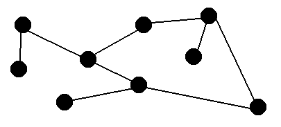
A graph is a data structure which allows us to model these kinds of relationships. A graph is a collection of vertices (such as major cities) and edges (roads between those major cities). Any collection of vertices and edges is a graph. For example, the following is a graph:

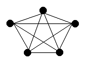
This graph does not demonstrate any noticeable pattern, but from certain points we can get to other points. Some graphs do have a recognizable pattern such as:

The first graph is what we call a complete or fully-connected graph. In a fully-connected graph, every vertex has an edge to every other vertex.

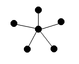
The graph on the right should seem familiar to you. If we bunch up all of the edges at the bottom so that the center is now on top, this should look strikingly similar to a generic tree. This is not a coincidence -- trees are graphs. In fact, they are a very specific type of graph: one without any cycles. A cycle is a sequence of edges that creates a path back to the vertex it starts at without reusing any of the edges.

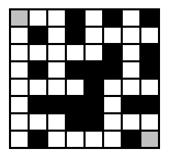
We used cities and roads as an example of what a graph might represent. Another common use for graphs is to model a maze.

In the case of a maze, the vertices represent each spot which you could ever be at, and the edges join those spots to all of the spots you could move to from there. As we will see, how you choose which spot to go to next could affect what path through the maze you eventually find.

Weighted Graphs

What if we wanted to go from Philadelphia to Charleston? We could go through Pittsburgh, but what if there is a better way? If we start out in a more southwestern direction, we might be able to find a faster route from Philadelphia to Charleston. On the other hand, while there might be a more direct path, the roads involved might be small slow roads, so the time that it takes might actually be longer even though the path is shorter.

In a graph, we can factor these details in when we are trying to find the best way to get from one place to another. Rather than simply indicating that there is an edge between two vertices, we will also give that edge a weight. If we are trying to find the fastest path from Philadelphia to Charleston, then the weight we use might be the expected time it takes on each part of the trip. If we are trying to find the shortest path, the weight we use might be the actual length of each part of the trip. We could also use some combination of these values.

We call this a weighted graph. For convenience, we will say that the weight will be infinity if there is no edge between two vertices, and that there will be a weight of 0 for staying at the current node.

Directed Graphs

Again returning to the road analogy, there is the concept of a one-way street. If you are at the Cathedral Of Learning and need to go to the highway, you have to use Fifth Ave., but if you are coming from the highway to the Cathedral Of Learning, you need to use Forbes Ave. instead, because both streets are one-way.

We might also want to have this type of behavior in our graph. We might want to be able to go from vertex A to vertex B directly, but not be able to go from vertex B to vertex A. We call this a directed graph. In a directed graph we say than an edge goes "from" one vertex "to" another vertex.

A directed graph can also be weighted. It might be really easy to go directly from vertex A to vertex B, but it might be very difficult (though possible) to go directly from vertex B to vertex A. In this case, there would be an edge from A to B and an edge from B to A, but the edge from B to A would have a much higher weight than the edge from A to B.

How Do We Represent Graphs?

Now that we understand what a graph is, how do we represent them on a computer. With the Linked List and the Binary Tree it was easy, but graphs are unstructured. One vertex might be adjecent to every other vertex, but another vertex might only be adjacent to just that one. (By adjacent, we mean that there is an edge between them, or that there is an edge from that one to the other in the case of a directed graph.)

There are two common ways of representing graphs. One is called an adjacency list, the other is called an adjacency matrix.

Adjacency List

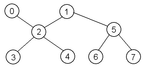
An adjacency list representation is essentially an array of linked lists, one for each vertex, where the linked list contains all of the vertices that are adjacent to a given vertex, and in the case of a weighted graph, the weight between that vertex and each of the others. Suppose we have the following graph (the naming of the vertices is arbitrary):

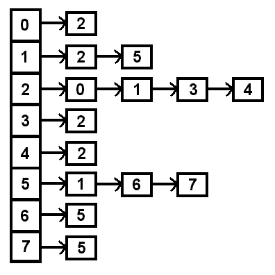
Then our adjacency list would look like:

Why is this? Well, vertex 0 only has an edge with vertex 2, but vertex 2 has edges with vertex 0, vertex 1, vertex 3, and vertex 4, so the only item in the list at index 0 is 2, while at index 2 the list contains 0, 1, 3, and 4. If this were a weighted graph, the nodes of the list would need to include both the number of the vertex and the cost to get there. If this were a directed graph, then an edge from 0 to 2 would not necessarily mean that there would be an edge from 2 to 0.

The following code implements an adjacency list which can be used for graphs that are either weighted or unweighted, and either directed or bidirected (the edges go in both directions).

class AdjList
{
	/*
	 * this class represents a weighted edge.  if the graph
	 * is unweighted, we will assign the weight of an existing
	 * edge to be 0
	 */
	private class Edge
	{
		private int vertex;
		private int cost;

		public Edge(int vertex, int cost)
		{
			this.vertex = vertex;
			this.cost = cost;
		}

		public Edge(int vertex)
		{
			this.vertex = vertex;
			this.cost = 0;
		}

		/*
		 * considers two edges equal if they go to the same
		 * vertex, regardless of their weight
		 */
		public boolean equals(Edge other_edge)
		{
			if (other_edge.vertex == this.vertex)
			{
				return true;
			}
			else
			{
				return false;
			}
		}
	}

	private LinkedList list[];
	private int num_vertices;

	public AdjList(int num_vertices)
	{
		this.num_vertices = num_vertices;
		list = new LinkedList[num_vertices];

		/*
		 * initialize all of the linked lists in the array
		 */
		for (int index = 0; index < num_vertices; index++)
		{
			list[index] = new LinkedList();
		}
	}

	/*
	 * add a directed weighted edge to the graph
	 */
	public addEdge(int vertex_from, int vertex_to, int cost)
	{
		list[vertex_from].addHead(new Edge(vertex_to, cost));
	}

	/*
	 * add a directed unweighted edge to the graph
	 */
	public addEdge(int vertex_from, int vertex_to)
	{
		addEdge(vertex_from, vertex_to, 0);
	}

	/*
	 * add a bidirected weighted edge to the graph
	 *
	 * to do this, we will add a directed edge in both directions
	 * with the same weight
	 */
	public addBidirectedEdge(int vertex_one, int vertex_two, int cost)
	{
		addEdge(vertex_one, vertex_two, cost);
		addEdge(vertex_two, vertex_one, cost);
	}

	/*
	 * add a bidirected unweighted edge to the graph
	 *
	 * to do this, we will add a directed edge in both directions
	 */
	public addBidirectedEdge(int vertex_one, int vertex_two)
	{
		addEdge(vertex_one, vertex_two, 0);
		addEdge(vertex_two, vertex_one, 0);
	}

	/*
	 * remove a directed edge from the graph
	 */
	public removeEdge(int vertex_from, int vertex_to)
	{
		list[vertex_from].remove(new Edge(vertex_to));
	}

	/*
	 * remove a bidirected edge from the graph
	 *
	 * to this, we will remove a directed edge in both directions
	 */
	public removeBidirectedEdge(int vertex_one, int vertex_two)
	{
		removeEdge(vertex_one, vertex_two);
		removeEdge(vertex_two, vertex_one);
	}

	/*
	 * return back the cost of a given edge
	 */
	public int getEdge(int vertex_from, int vertex_to)
	{
		Edge foundEdge = list[vertex_from].find(new Edge(vertex_to));

		if (null == foundEdge)
		{
			return Integer.MAX_VALUE;
		}
		else
		{
			return foundEdge.cost;
		}
	}
}

Adjacency Matrix

Another way we can represent a graph is by using an adjacency matrix. An adjacency matrix is a table which tells us if there is an edge between two vertices, and in the case of a weighted graph, the weight of the edge.

If there are N vertices in the graph, the adjacency matrix will be an N x N array of integers, where the rows represent the "from" end of the edge, and the columns represent the "to" end of the edge. The entry at (i, j) contains the weight of the edge from vertex #i to vertex #j, or infinity if no such edge exists. In the case of a bidirectional graph, if there is an edge from vertex #i to vertex #j there is also an edge from vertex #j to vertex #i, so the adjacency matrix will be symmetric.

Let's take another look at the graph we used for the adjacency list:

The adjacency matrix for this graph would be:

	0	1	2	3	4	5	6	7
0	0	-	0	-	-	-	-	-
1	-	0	0	-	-	0	-	-
2	0	0	0	0	0	-	-	-
3	-	-	0	0	-	-	-	-
4	-	-	0	-	0	-	-	-
5	-	0	-	-	-	0	0	0
6	-	-	-	-	-	0	0	-
7	-	-	-	-	-	0	-	0

Above, "-" means that there is no edge there (the value is infinity).

In this case, the graph was bidirectional, so if you look along the diagonal, you will see that the matrix is, in fact, symmetric. If this were a large graph with many vertices, we could save space by only storing the upper or lower triangle, and use those values as both index (i, j) and index (j, i).

Also, if you look at this matrix, you will see that we have 0's along the diagonal, which suggests that vertices are adjacent to themselves. This is implementation specific -- depending on what you are trying to represent, you may or may not want to let vertices be adjacent to themselves.

Now, let's take a look at code to implement an adjacency matrix. We will implement the same methods that the AdjList class has.

class AdjMatrix
{
	private int [][] matrix;
	private int num_vertices;

	private const int inf = Integer.MAX_VALUE;

	public AdjMatrix(int num_vertices)
	{
		this.num_vertices = num_vertices;
		matrix = new int[num_vertices][num_vertices];

		// let's assume that nodes are adjacent to themselves
		for (int vertex = 0; vertex < num_vertices; vertex++)
		{
			for (int other_vertex = 0; other_vertex < num_vertices; other_vertex++)
			{
				if (other_vertex == vertex)
				{
					matrix[vertex][other_vertex] = 0;
				}
				else
				{
					matrix[vertex][other_vertex] = inf;
				}
			}
		}
	}

	public void addEdge(int vertex_from, int vertex_to, int cost)
	{
		matrix[vertex_from][vertex_to] = cost;
	}

	public void addEdge(int vertex_from, int vertex_to)
	{
		addEdge(vertex_from, vertex_to, 0);
	}

	public void addBidirectedEdge(int vertex_one, int vertex_two, int cost)
	{
		addEdge(vertex_one, vertex_two, cost);
		addEdge(vertex_two, vertex_one, cost);
	}

	public void addBidirectedEdge(int vertex_one, int vertex_two)
	{
		addEdge(vertex_one, vertex_two, 0);
		addEdge(vertex_two, vertex_one, 0);
	}

	public removeEdge(int vertex_from, int vertex_to)
	{
		matrix[vertex_from][vertex_to] = inf;
	}

	public removeBidirectedEdge(int vertex_one, int vertex_two)
	{
		matrix[vertex_one][vertex_two] = inf;
		matrix[vertex_two][vertex_one] = inf;
	}

	public int getEdge(int vertex_from, int vertex_to)
	{
		return matrix[vertex_from][vertex_to];
	}
}
	

Lists Vs. Matrices

We have two ways to represent graphs, so which one should we use?

Well, if the graph is sparse (there aren't many edges), then the matrix will take up a lot of space indication all of the pairs of vertices which don't have an edge between them, but the adjacency list does not have that problem, because it only keeps track of what edges are actually in the graph. On the other hand, if there are a lot of edges in the graph, or if it is fully connected, then the list has a lot of overhead because of all of the references.

If we need to look specifically at a given edge, we can go right to that spot in the matrix, but in the list we might have to traverse a long linked list before we hit the end and find out that it is not in the graph.

On the other hand, if we need to look at all of a vertex's neighbors, if you use a matrix you will have to scan through all of the vertices which aren't neighbors as well, whereas in the list you can just scan the linked-list of neighbors.

If, in a directed graph, we ask the question, "Which verticies have edges leadingt to vertex X?", the answer is straight-forward to find in an adjacency matrix -- we just walk down column X and report all of the edges that are present. But, life isn't so easy with the adjacency list -- we actually have to perform a brute-force search.

So which representation you use depends on what you are trying to represent and what you plan on doing with the graph.